
Taxon-set enrichment analysis with TaxSEA
Last updated on 2026-04-28 | Edit this page
Estimated time: 20 minutes
Overview
Questions
- How can we test whether groups of related taxa (taxon sets) show coordinated shifts between conditions?
- What input does TaxSEA need, and how should taxonomic IDs be formatted?
- How does TaxSEA extend differential abundance results using enrichment analysis?
- How can we interpret enriched taxon sets to understand functional, ecological, or disease-associated patterns?
Objectives
- Prepare species- or genus-level differential abundance results for use with TaxSEA.
- Run TaxSEA to test for enrichment across predefined or custom taxon sets.
- Understand the structure of TaxSEA output, including P values, effect direction, and FDR.
- Interpret enrichment results in the context of microbiome function, ecology, and host associations.
Authors: Calum J. Walsh & Feargal J. Ryan
TaxSEA is a Bioconductor package that helps microbiome researchers test for enrichment in known microbial signatures, including:
- Metabolite producers
- Disease associations
- Previously published microbiome signatures
- Traits established from in-vitro data
TaxSEA takes as input a vector of genus or species names and a rank (e.g. log2 fold changes or Spearman’s rho) and uses a Kolmogorov-Smirnov test to identify if a particular group of species or genera (i.e. a set of taxa such as butyrate producers) are skewed to one end of the distribution (i.e. enriched).
TaxSEA is based on the concept of Gene Set Enrichment Analysis (GSEA). For an overview, check out the link here:https://www.metwarebio.com/gsea-enrichment-analysis-guide/.
Note: Although TaxSEA can, in principle, be applied to microbiome data from any source, the databases utilised largely cover human-associated microbiomes, particularly the human gut microbiome. As such TaxSEA will likely perform best on human gut microbiome data.
Taxon set database
By default TaxSEA utilises taxon sets generated from reference databases (gutMGene, GMrepo v2, MiMeDB, mBodyMap, BugSigDB, BacDive) as well as a handful of sets curated from the literature (mucin utilisers and BLOSSUM taxa). See below for examples of using custom databases or taxonomically-defined taxon sets.
Please cite the appropriate database if using:
- Cheng et al. gutMGene: a comprehensive database for target genes of gut microbes and microbial metabolites Nucleic Acids Res. 2022.
- Dai et al. GMrepo v2: a curated human gut microbiome database with special focus on disease markers and cross-dataset comparison Nucleic Acids Res. 2022.
- Wishart et. al. MiMeDB: the Human Microbial Metabolome Database Nucleic Acids Res. 2023.
- Jin et al. mBodyMap: a curated database for microbes across human body and their associations with health and diseases. Nucleic Acids Res. 2022.
- Geistlinger et al. BugSigDB captures patterns of differential abundance across a broad range of host-associated microbial signatures. Nature Biotech. 2023.
Load the Package
R
library(TaxSEA)
Input
All that is required for TaxSEA is an R vector containing ranks (e.g. log2 fold changes) and names (e.g. species/genus). TaxSEA will not work if input names are from ranks higher than species or genus and will struggle with GTDB taxonomy. The input should include all taxa tested, not a limited or pre-defined set (e.g. do not use a threshold for significance or remove any taxa). TaxSEA will lookup and convert taxon names to NCBI taxonomic identifiers. TaxSEA stores a commonly observed identifiers internally and so will only lookup whatever is not covered to save time.
Input IDs should be formatted like one of the following:
- Species name. E.g. “Bifidobacterium longum”, “Bifidobacterium_longum”
- Genus name. E.g. “Bifidobacterium”
- NCBI ID E.g. “216816”
The code chunk below is useful for splitting names that contain the full species taxonomy (eg. MetaPhlAn output). We don’t need to run it now.
R
# Input IDs with the full taxonomic lineage should be split E.g.
x <- "d__Bacteria.p__Actinobacteriota.c__Actinomycetes.o__Bifidobacteriales.f__Bifidobacteriaceae.g__Bifidobacterium"
x <- strsplit(x, split = "\\.")[[1]][6]
x <- gsub("g__", "", x)


# Running this through a vector of IDs may look something like the following
new_ids <- sapply(as.character(old_ids), function(y) {strsplit(x = y, split = "\\.")[[1]][6]})
new_ids <- gsub("g__", "", new_ids)
Load and Inspect Test Data
The TaxSEA library comes with pre-processed test data included.
The data comes from a study comparing
IBD patients to healthy controls.
The count data was downloaded from curatedMetagenomicData
and fold changes between the two groups were generated with LinDA.
We can load this data into our working environment using the
data() function
R
data("TaxSEA_test_data")

sample(TaxSEA_test_data, 4)
OUTPUT
 Haemophilus_sp_HMSC71H05          Dorea_sp_CAG_317 Monoglobus_pectinilyticus
                    2.179                     2.162                    -1.069
     Actinomyces_sp_ICM47
                    1.539
The input is a vector of species names and log fold changes. Perfect for TaxSEA.
Run TaxSEA with Test Data
R
taxsea_results <- TaxSEA(taxon_ranks = TaxSEA_test_data)
Examine outputs
Output
The output is a list of data frames providing enrichment results for metabolite produers, health/disease associations, and published signatures from BugSigDB. Each dataframe has at least 6 columns:
- taxonSetName - The name of the taxon set tested
- median_rank_of_set_members - This is simply the median rank across all detected members in the set. This allows you to see the direction of change
- PValue - Kolmogorov-Smirnov test P value.
- Test_statistic - Kolmogorov-Smirnov test statistic.
- FDR - P value adjusted for multiple testing.
- TaxonSet - Returns list of taxa in the set to show what is driving the signal
All results: This includes all databases. Is useful for a quick look and overview but can get a bit messy.
R
all_results.df <- taxsea_results$All_databases
Metabolite Producers: Enrichment among metabolite producers from gutMgene and MiMeDB
R
metabolites.df <- taxsea_results$Metabolite_producers
Health Associations: Enrichment among health and disease signatures from GMRepoV2 and mBodyMap
R
disease.df <- taxsea_results$Health_associations
BugSigDB: Enrichment among published associations from BugSigDB - a database of manually curated microbial signatures from published differential abundance studies. The output format here is a bit different. You’ll notice that, where available, it includes a PubMed ID linking back to the reporting paper.
R
bsdb.df <- taxsea_results$BugSigDB
Bacterial Physiology: Enrichment among bacterial meta data from from BacDive - a standardised database of bacterial information, including physiology.
R
bacdive.df <- taxsea_results$BacDive_bacterial_physiology
Visualisation of TaxSEA output
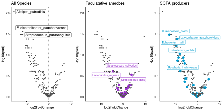
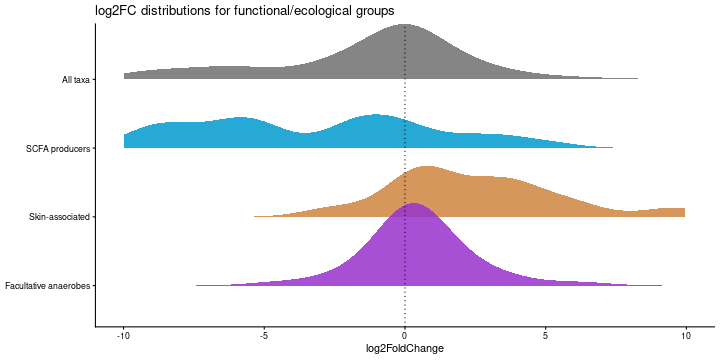
As TaxSEA operates on individual species and ranks, the easiest way to visualise these is often through the input ranks. For example using volcano plots, or density plots can be intuitive and useful ways to see the overall trend in a set and the members driving it. Remember just becomes an individual species isn’t significant by itself, doesn’t mean that the set cannot be significant.
R
library(ggplot2)
library(gridExtra)
library(reshape)
library(curatedMetagenomicData)
library(TaxSEA)
library(MicrobiomeStat)
library(ggrepel)
library(ggpubr)
library(ggridges)

########################
#### HallAB_2017 ####
########################
allmeta_data = sampleMetadata

# HallAB_2017 dataset
HallAB_2017_cmd_object = curatedMetagenomicData(pattern = "2021-10-14.HallAB_2017.relative_abundance",counts = TRUE,dryrun = FALSE)
R
HallAB_2017_counts.df = HallAB_2017_cmd_object
HallAB_2017_counts.df = (HallAB_2017_counts.df$`2021-10-14.HallAB_2017.relative_abundance`)

HallAB_2017_counts.df = assay(HallAB_2017_counts.df)
HallAB_2017_counts.df = HallAB_2017_counts.df[apply(HallAB_2017_counts.df>1000,1,sum)>4,]
HallAB_2017_md.df = allmeta_data[allmeta_data$sample_id %in% colnames(HallAB_2017_counts.df),]
rownames(HallAB_2017_md.df) = HallAB_2017_md.df$sample_id

## Ensure data is matching
colnames(HallAB_2017_counts.df) %in% rownames(HallAB_2017_md.df)
OUTPUT
  [1] TRUE TRUE TRUE TRUE TRUE TRUE TRUE TRUE TRUE TRUE TRUE TRUE TRUE TRUE TRUE
 [16] TRUE TRUE TRUE TRUE TRUE TRUE TRUE TRUE TRUE TRUE TRUE TRUE TRUE TRUE TRUE
 [31] TRUE TRUE TRUE TRUE TRUE TRUE TRUE TRUE TRUE TRUE TRUE TRUE TRUE TRUE TRUE
 [46] TRUE TRUE TRUE TRUE TRUE TRUE TRUE TRUE TRUE TRUE TRUE TRUE TRUE TRUE TRUE
 [61] TRUE TRUE TRUE TRUE TRUE TRUE TRUE TRUE TRUE TRUE TRUE TRUE TRUE TRUE TRUE
 [76] TRUE TRUE TRUE TRUE TRUE TRUE TRUE TRUE TRUE TRUE TRUE TRUE TRUE TRUE TRUE
 [91] TRUE TRUE TRUE TRUE TRUE TRUE TRUE TRUE TRUE TRUE TRUE TRUE TRUE TRUE TRUE
[106] TRUE TRUE TRUE TRUE TRUE TRUE TRUE TRUE TRUE TRUE TRUE TRUE TRUE TRUE TRUE
[121] TRUE TRUE TRUE TRUE TRUE TRUE TRUE TRUE TRUE TRUE TRUE TRUE TRUE TRUE TRUE
[136] TRUE TRUE TRUE TRUE TRUE TRUE TRUE TRUE TRUE TRUE TRUE TRUE TRUE TRUE TRUE
[151] TRUE TRUE TRUE TRUE TRUE TRUE TRUE TRUE TRUE TRUE TRUE TRUE TRUE TRUE TRUE
[166] TRUE TRUE TRUE TRUE TRUE TRUE TRUE TRUE TRUE TRUE TRUE TRUE TRUE TRUE TRUE
[181] TRUE TRUE TRUE TRUE TRUE TRUE TRUE TRUE TRUE TRUE TRUE TRUE TRUE TRUE TRUE
[196] TRUE TRUE TRUE TRUE TRUE TRUE TRUE TRUE TRUE TRUE TRUE TRUE TRUE TRUE TRUE
[211] TRUE TRUE TRUE TRUE TRUE TRUE TRUE TRUE TRUE TRUE TRUE TRUE TRUE TRUE TRUE
[226] TRUE TRUE TRUE TRUE TRUE TRUE TRUE TRUE TRUE TRUE TRUE TRUE TRUE TRUE TRUE
[241] TRUE TRUE TRUE TRUE TRUE TRUE TRUE TRUE TRUE TRUE TRUE TRUE TRUE TRUE TRUE
[256] TRUE TRUE TRUE TRUE
R
HallAB_2017_counts.df = HallAB_2017_counts.df[,rownames(HallAB_2017_md.df)]
HallAB_2017_md.df = HallAB_2017_md.df[,c("study_name","sample_id","subject_id","study_condition","age_category","DNA_extraction_kit","visit_number")]

## Remove duplicate samples
HallAB_2017_md.df = HallAB_2017_md.df[order(HallAB_2017_md.df$visit_number,decreasing = FALSE),]
HallAB_2017_md.df = HallAB_2017_md.df[!duplicated(HallAB_2017_md.df$subject_id),]
HallAB_2017_counts.df = HallAB_2017_counts.df[,rownames(HallAB_2017_md.df)]

## Assigning rows as species names ##
spec_vec = sapply(as.character(rownames(HallAB_2017_counts.df)),function(y) {strsplit(x = y,split="\\|")[[1]][7]})
names(spec_vec) = NULL
spec_vec = gsub("s__","",spec_vec)
rownames(HallAB_2017_counts.df) = spec_vec

HallAB_2017_linda_res = linda(HallAB_2017_counts.df,
                              HallAB_2017_md.df,
                              formula = '~study_condition+DNA_extraction_kit')
OUTPUT
0  features are filtered!
The filtered data has  32  samples and  299  features will be tested!
OUTPUT
Imputation approach is used.
Fit linear models ...
Completed.
R
HallAB_2017_ranks = HallAB_2017_linda_res$output$study_conditionIBD$log2FoldChange
names(HallAB_2017_ranks) = rownames(HallAB_2017_linda_res$output$study_conditionIBD)
HallAB_2017_TaxSEA_results.df = TaxSEA(taxon_ranks = HallAB_2017_ranks)

alldb = HallAB_2017_TaxSEA_results.df$All_databases
HallAB_2017_DA = HallAB_2017_linda_res$output$study_conditionIBD

hall_bacterialids = get_ncbi_taxon_ids(rownames(HallAB_2017_DA))
data("TaxSEA_db")

scfas = unique(unlist(c(TaxSEA_db$GutMGene_producers_of_Propionate,
                        TaxSEA_db$GutMGene_producers_of_Butyrate)))

HallAB_2017_DA$NCBI_id = hall_bacterialids[rownames(HallAB_2017_DA)]
HallAB_2017_DA$Nitrate_utilisers = HallAB_2017_DA$NCBI_id %in% TaxSEA_db$BacDive_Utilizes_nitrate
HallAB_2017_DA$Faculatative_anerobes = HallAB_2017_DA$NCBI_id %in% TaxSEA_db$`BacDive_facultative anaerobe`
HallAB_2017_DA$SCFA_producers = HallAB_2017_DA$NCBI_id %in% scfas
HallAB_2017_DA$Species = rownames(HallAB_2017_DA)
HallAB_2017_DA$mBodyMap_skin = HallAB_2017_DA$NCBI_id %in% TaxSEA_db$mBodyMap_skin


volcano_plot_all = ggplot(HallAB_2017_DA,aes(x=log2FoldChange,y=-log10(padj)))+
  geom_point(color="grey33",size=1)+
  theme_classic()+guides(color="none",size="none")+
  geom_label_repel(data=HallAB_2017_DA[HallAB_2017_DA$padj < 0.1,],
                   aes(label=Species))+
  geom_vline(xintercept = 0,linetype=3)+
  geom_hline(yintercept = -log10(0.1),linetype=3)+
  ggtitle("All Species")


scfa_volcano = ggplot(HallAB_2017_DA,aes(x=log2FoldChange,y=-log10(padj),
                               colour=SCFA_producers,
                               size=SCFA_producers))+
  geom_point()+
  scale_colour_manual(values=c("grey33","deepskyblue3"))+
  scale_size_manual(values=c(1,3))+
  theme_classic()+guides(color="none",size="none")+
  geom_label_repel(data=HallAB_2017_DA[HallAB_2017_DA$SCFA_producers==TRUE,],
                   aes(label=Species),max.overlaps = 4)+
  ggtitle("SCFA producers")


volcano_fa = ggplot(HallAB_2017_DA,aes(x=log2FoldChange,y=-log10(padj),
                               colour=Faculatative_anerobes,
                               size=Faculatative_anerobes))+
  geom_point()+
  scale_colour_manual(values=c("grey33","darkorchid"))+
  scale_size_manual(values=c(1,3))+
  theme_classic()+guides(color="none",size="none")+
  geom_label_repel(data=HallAB_2017_DA[HallAB_2017_DA$Faculatative_anerobes==TRUE,],
                   aes(label=Species))+
  ggtitle("Faculatative anerobes")

ggarrange(volcano_plot_all,volcano_fa,scfa_volcano,ncol = 3,nrow=1)
R
 ## Build a long df for the ridge plot
 ridge_dat <- rbind(
   data.frame(log2FoldChange = HallAB_2017_DA$log2FoldChange,
              Group = "All taxa"),
   data.frame(log2FoldChange = HallAB_2017_DA$log2FoldChange[HallAB_2017_DA$SCFA_producers],
              Group = "SCFA producers"),
   data.frame(log2FoldChange = HallAB_2017_DA$log2FoldChange[HallAB_2017_DA$mBodyMap_skin],
              Group = "Skin-associated"),
   data.frame(log2FoldChange = HallAB_2017_DA$log2FoldChange[HallAB_2017_DA$Faculatative_anerobes],
              Group = "Facultative anaerobes")
 )

 ridge_dat$Group <- factor(
   ridge_dat$Group,
   levels = rev(c("All taxa",
                  "SCFA producers",
                  "Skin-associated",
                  "Facultative anaerobes"))
 )

 ggplot(ridge_dat,
        aes(x = log2FoldChange,
            y = Group,
            fill = Group)) +
   geom_density_ridges(alpha = 0.85, scale = 1.2, colour = NA) +
   xlim(-10, 10) +
   geom_vline(xintercept = 0, linetype = 3) +
   theme_classic() +
   scale_fill_manual(values = rev(c(
     "grey44",        # All taxa
     "deepskyblue3",  # SCFA
     "tan3",          # Skin
     "darkorchid"     # Anaerobes
   ))) +
   theme(legend.position = "none") +
   ylab(NULL) +
   ggtitle("log2FC distributions for functional/ecological groups")
Custom databases
If you want to run TaxSEA with your own database, use the
custom_db argument. It should be a named list where:
- each name is the label for a set, and
- each value is a vector of species assigned to that set.
This is the same format as the default TaxSEA database.
Note: using the custom_db flag disables the automatic ID conversion and NCBI API lookup. However this is available via other functions.
Perform enrichment analysis using TaxSEA with custom databases
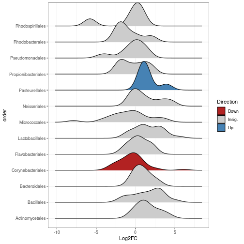
In addition to taxon sets defined by function or phenotype, users can define custom sets based on taxonomy. Current methods to test differential abundance at higher taxonomic levels (e.g., genus or family) involve aggregating counts, but with this approach opposing shifts in individual species may cancel each other out, obscuring meaningful biological patterns. For instance, antibiotic treatment may suppress certain species while allowing resistant species within the same genus to expand and occupy the vacant niche, creating an ecological shift that appears as no net change at broader taxonomic levels. Here we utilise data from Chng et al. 2016, a study comparing the skin microbiome between Atopic dermatitis and controls.
The script below applies the TaxSEA framework to identify taxonomic enrichment at different taxonomic levels. Specifically, we analyse enrichment at the order level from metagenomic data.
The code block below does the following:
- Downloads species abundance data
- Performs some light QC
- Defines taxonomic sets at each level of taxonomy (phylum -> genus)
- Calculates differential abundance between groups
- Performs enrichment analysis using TaxSEA
- Plots results
R
# Load required libraries
library(TaxSEA)
library(curatedMetagenomicData)
library(tidyverse)
library(phyloseq)
library(MicrobiomeStat)
library(dplyr)
library(DT)

# Load sample metadata from curatedMetagenomicData
metadata_all <- sampleMetadata

# Filter metadata for the specific study (ChngKR_2016)
metadata <- metadata_all %>%
  filter(study_name == "ChngKR_2016") %>%
  column_to_rownames('sample_id')

# Extract count data from curatedMetagenomicData
cmd_data <- curatedMetagenomicData(
  pattern = "ChngKR_2016.relative_abundance",
  counts = TRUE,
  dryrun = FALSE
)
R
# Convert the extracted data to a count matrix
counts_data <- assay(cmd_data[[1]])
# Subset to relevant samples
counts_data <- counts_data[, rownames(metadata)]

# Filter taxa to only keep those with at least one sample having counts > 100
counts_data <- counts_data[apply(counts_data > 100, 1, sum) > 0, ]

# Extract species names from taxonomic strings
species_names <- gsub("s__", "", sapply(rownames(counts_data), function(y) strsplit(y, "\\|")[[1]][7]))
rownames(counts_data) <- species_names

# Create a taxonomic lineage data frame to define Sets
# Remove taxonomic prefixes (k__, p__, c__, etc.) and separate into taxonomic ranks
taxon_lineages <- data.frame(Name = species_names,
                             Lineage = names(species_names)) %>%
  mutate(Lineage = str_remove_all(Lineage, '[kpcofgs]__')) %>%
  separate(col = Lineage, into = c('kingdom', 'phylum', 'class',
                                   'order', 'family', 'genus', 'species'),
           sep = '\\|') %>%
  mutate(name = Name) %>%
  remove_rownames() %>%
  column_to_rownames('name')

# Perform differential abundance testing using LinDA
metadata$study_condition <- factor(metadata$study_condition, levels = c("control", "AD"))

linda_results <- linda(
  feature.dat = counts_data,
  meta.dat = metadata,
  formula = '~study_condition',
  feature.dat.type = 'count',
  prev.filter = 0.05
)
OUTPUT
216  features are filtered!
The filtered data has  78  samples and  216  features will be tested!
Pseudo-count approach is used.
Fit linear models ...
Completed.
R
# Extract log2 fold change values for differential taxa
linda_results <- linda_results$output$study_conditionAD
log2_fold_changes <- linda_results$log2FoldChange
names(log2_fold_changes) <- rownames(linda_results)


# Create a named list of species grouped by order
custom_taxon_sets <- taxon_lineages %>%
  group_by(.data[['order']]) %>%
  summarise(species = list(species), .groups = "drop") %>%
  deframe()

# Perform enrichment analysis using TaxSEA
custom_taxsea_results <- TaxSEA(taxon_ranks = log2_fold_changes, custom_db = custom_taxon_sets)
custom_taxsea_results <- custom_taxsea_results$custom_sets

datatable(custom_taxsea_results)
R
# plotting
data.frame(Name = names(log2_fold_changes),
           Log2FC = log2_fold_changes) %>%
  left_join(taxon_lineages) %>%
  left_join(custom_taxsea_results, by = c("order" = "taxonSetName")) %>%
  mutate(Direction = if_else(FDR > 0.1, 'Insig.', if_else(median_rank_of_set_members > 0, 'Up', 'Down'))) %>%
  drop_na(PValue) %>%
  ggplot(aes(x = Log2FC, y = order, group = order)) +
  geom_density_ridges(aes(fill = Direction)) +
  theme_bw() +
  scale_fill_manual(values = c('Insig.' = 'grey80',
                              'Up' = 'steelblue',
                              'Down' = 'firebrick'))
- TaxSEA performs taxon-set enrichment analysis on differential abundance results, similar to GSEA.
- Inputs must be species or genus names with corresponding ranks (e.g., log2 fold changes).
- TaxSEA tests whether members of a taxon set are skewed toward one end of the ranked distribution.
- Enrichment results help reveal functional or ecological patterns that may not be visible at the single-taxon level.