
All in One View
Content from Background
Last updated on 2026-10-06 | Edit this page
Overview
Questions
- Why is the fat‑tailed dunnart a useful model for microbiome studies?
- What are the expected experimental differences between captive and wild animals?
- Why use a byobu / screen session on a remote instance?
- What are symbolic links and why are they used here?
Objectives
- Place the dataset in ecological and conservation context.
- Relate host ecology and sample provenance to interpretation of microbiome results.
- Launch and reconnect to a persistent byobu‑screen session.
- Create symbolic links to shared tutorial data to avoid redundant copies.
What is the influence of captivity on gut microbiota of the fat-tailed dunnart?
The Players
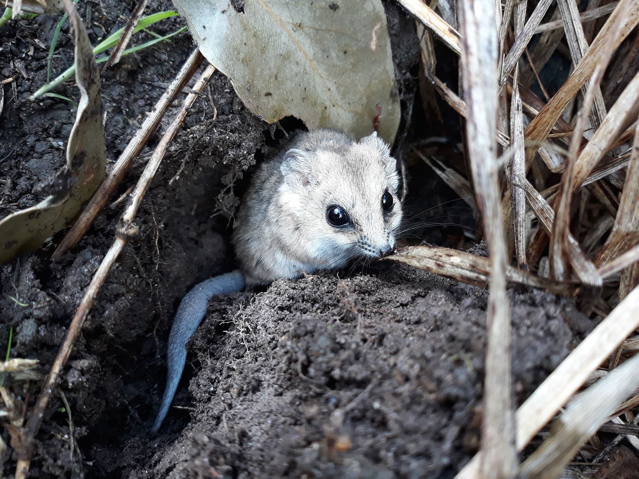 (Photo credit: Emily
Scicluna)
(Photo credit: Emily
Scicluna)
- Fat-tailed dunnart Sminthopsis crassicaudata - a species of mouse-like marsupial in the family Dasyuridae, which includes quolls, the Tasmanian devil, and the extinct Thylacine. There are 10 samples in this dataset (This data is a subset from a larger experiment); 5 faecal samples each from captive and wild fat-tailed dunnarts.
The Study
Indigenous microbial communities (microbiota) play critical roles in host health. Small marsupials, such as the fat-tailed dunnart, are increasingly used as model systems to understand how environmental conditions shape host-associated microbiomes. Transitions between wild and captive environments can substantially alter diet, behaviour, and microbial exposure, providing a natural framework to investigate microbiome restructuring and its potential consequences for host physiology and health. Here, we characterise the gut microbiome of wild and captive fat-tailed dunnarts to assess how captivity influences microbial community composition. This dataset represents a subset of a larger experimental framework examining microbiome-mediated effects on host function and conservation outcomes.
QIIME 2 Analysis platform
The version used in this workshop is qiime2-2026.1.
Other versions of QIIME2 may result in minor differences in results.
Quantitative Insights Into Microbial Ecology 2 (QIIME 2™) is a next-generation microbiome bioinformatics platform that is extensible, free, open source, and community developed. It allows researchers to:
- Automatically track analyses with decentralised data provenance
- Interactively explore data with beautiful visualisations
- Easily share results without QIIME 2 installed
- Plugin-based system — researchers can add in tools as they wish
Viewing QIIME2 visualisations
In order to use QIIME2 View to visualise your files, you will need to use a Google Chrome or Mozilla Firefox web browser (not in private browsing). For more information, click here.
As this workshop is being run on a remote Nectar Instance, you will need to download the visual files (*.qzv) to your local computer and view them in QIIME2 View (q2view).
We will be doing this step multiple times throughout this workshop to view visualisation files as they are generated.
Alternatively, if you have QIIME2 installed and are
running it on your own computer, you can use
qiime tools view to view the results from the command line
(e.g. qiime tools view filename.qzv).
qiime tools view opens a browser window with your
visualization loaded in it. When you are done, you can close the browser
window and press ctrl-c on the keyboard to terminate the
command.
- Captivity can alter diet, exposure and behaviour — all of which may reshape the gut microbiome.
- The dataset contains a small, balanced subset (5 captive, 5 wild) suitable for teaching and demonstrating methods.
- Use byobu-screen to keep long‑running commands alive across disconnections.
- Symlinks point to /mnt/shared_data to conserve storage and keep everyone working from the same files.
Content from Importing, cleaning and quality control of the data
Last updated on 2026-10-06 | Edit this page
Overview
Questions
- How do you import demultiplexed paired‑end FASTQ files into a QIIME 2 artefact?
- Why must primers be removed prior to denoising?
- What diagnostics should you inspect before selecting DADA2 truncation parameters?
Objectives
- Import Casava‑formatted demultiplexed paired‑end reads into a single SampleData artefact.
- Remove primers with cutadapt while handling degenerate bases and quality trimming.
- Generate demux quality summaries and choose appropriate DADA2 truncation lengths to balance read quality and merge overlap.
Import data
These samples were sequenced on a single Illumina NextSeq run at the Walter and Eliza Hall Institute (WEHI), Melbourne, Australia. Data from WEHI came as paired-end, demultiplexed, unzipped *.fastq files with adapters still attached. Following the QIIME2 importing tutorial, this is the Casava One Eight format. The files have been renamed to satisfy the Casava format as SampleID_FWDXX-REVXX_L001_R[1 or 2]_001.fastq e.g. CTRLA_Fwd04-Rev25_L001_R1_001.fastq.gz. The files were then zipped (.gzip).
Here, the data files (two per sample i.e. forward and reverse reads
R1 and R2 respectively) will be imported and
exported as a single QIIME 2 artefact file. These samples are already
demultiplexed (i.e. sequences from each sample have been written to
separate files), so a metadata file is not initially required.
To check the input syntax for any QIIME2 command, enter the command,
followed by --help
e.g. qiime tools import --help
If you haven’t already done so, make sure you are running the workshop in byobu-screen and have created the symbolic links to the workshop data.
Start by making a new directory analysis to store all
the output files from this tutorial. In addition, we will create a
subdirectory called seqs to store the exported
sequences.
Run the command to import the raw data located in the directory
raw_data and export it to a single QIIME 2 artefact file,
combined.qza.
Remove primers
Remember to ask your sequencing facility if the raw data you get has the primers attached - they may have already been removed.
These sequences still have the primers attached and must be removed prior to denoising. For this workshop, primer trimming was performed using the QIIME 2 cutadapt trim-paired plugin to maintain a fully reproducible workflow within the QIIME 2 framework. Amplicons were generated using standard 16S rRNA gene primers for the v4 region, and the reads returned from the sequencer therefore include these primer sequences at the 5′ ends. Using cutadapt, the specified primer sequence and any bases upstream of the match are removed, with an error rate of 0.10 to balance sensitivity of primer detection with specificity of trimming. Degenerate bases in the primers are accommodated using wildcard matching, and any reads lacking the expected primer sequences are discarded to minimise inclusion of off-target amplification products. A modest 3′ quality trimming threshold (Phred score = 20) is also applied to remove low-quality bases prior to downstream denoising.
It is important to note that these data were generated on an Illumina NextSeq platform, which uses 2-colour chemistry and can produce artificial poly-G tails at the ends of reads under low-signal conditions. The QIIME 2 implementation of cutadapt does not have the –nextseq-trim parameter, which is specifically designed to remove these artefacts. As such, the trimming approach used here represents a simplified, self-contained workflow appropriate for teaching purposes. For production analyses of NextSeq data, best practice is to perform trimming with standalone cutadapt (including –nextseq-trim) prior to importing reads into QIIME 2, as this improves removal of sequencing artefacts and can enhance downstream denoising and taxonomic resolution.
BASH
qiime cutadapt trim-paired \
  --i-demultiplexed-sequences analysis/seqs/combined.qza \
  --p-front-f GTGYCAGCMGCCGCGGTAA \
  --p-front-r GGACTACNVGGGTWTCTAAT \
  --p-error-rate 0.10 \
  --p-overlap 10 \
  --p-match-adapter-wildcards \
  --p-discard-untrimmed \
  --p-quality-cutoff-3end 20 \
  --p-quality-cutoff-5end 0 \
  --p-cores 8 \
  --output-dir analysis/seqs_trimmed \
--verboseThe primers specified are the Earth Microbiome Project (EMP) 16S V4 primers (515F (Parada)– 806R (Apprill) targeting the v4 region of the bacterial 16S rRNA gene), which correspond to this specific experiment. Unless you are using these exact primers for your experiment, you need to adapt the code accordingly.
The error rate, --p-error-rate, and overlap,
--p-overlap, parameters will likely need to be adjusted for
your own sample data to maximise the proportion of reads successfully
trimmed while avoiding nonspecific matches. Play around with these
values and see what happens.
Create and interpret sequence quality data
Create a viewable summary file so the data quality can be checked. Viewing the quality plots generated here helps determine settings for dada2, which we will run next.
Trimmed sequences are processed using the dada2 plugin within
QIIME2. dada2 denoises data by modelling and correcting Illumina
amplicon sequencing errors, and infers exact amplicon sequence variants
(ASVs), resolving differences of as little as a single nucleotide. Its
workflow includes filtering, dereplication, paired-end read merging, and
reference-free chimera detection, resulting in a feature (ASV)
table.
Truncation removes bases from the 3′ end of reads at the specified position. When choosing DADA2 truncation lengths, the first step is to inspect the forward and reverse quality plots you just created. In many modern Illumina datasets, especially after primer and basic quality trimming, these plots may appear relatively flat with consistently high quality across most of the read length. In these cases, there is no obvious “cut point” where quality sharply declines. Instead of looking for a specific quality threshold (for example, Q35), you should choose truncation lengths conservatively, trimming only the very ends of reads if needed while retaining as much high-quality sequence as possible without compromising read overlap.
For paired-end data, an additional and critical consideration is read overlap. After truncation, the forward and reverse reads must still overlap sufficiently to merge. While the absolute minimum overlap is ~12 bp, an overlap of ~50 bp is recommended to ensure robust merging and reduce the risk of losing reads during this step. As a result, truncation lengths are often chosen by balancing two factors: maintaining high-quality sequence and preserving enough overlap for successful merging.
TL;DR: when quality plots are essentially straight lines, truncation is less about identifying where quality drops and more about keeping as much usable sequence as possible while ensuring adequate overlap between reads.
Things to look for when choosing truncation lengths
- Do the forward and reverse quality profiles show a clear decline near the ends of the reads? If so, truncate before the low-quality tail.
- If the quality profiles remain high and relatively flat, avoid trimming too aggressively and retain as much high-quality sequence as possible.
- Will the chosen forward and reverse truncation lengths still leave enough overlap for paired-end merging? A minimum overlap of ~50 bp is recommended.
Create a subdirectory in analysis called
visualisations to store all files that we will visualise in
one place.
BASH
qiime demux summarize \
--i-data analysis/seqs_trimmed/trimmed_sequences.qza \
--o-visualization analysis/visualisations/trimmed_sequences.qzvVisualisations: Read quality and demux output
Copy analysis/visualisations/trimmed_sequences.qzv to
your local computer and view in QIIME
2 View (q2view).
Click
to view the trimmed_sequences.qzv file in
QIIME 2 View.
Make sure to switch between the “Overview” and “Interactive Quality Plot” tabs in the top left hand corner. Click and drag on the plot to zoom in. Double click to zoom back out to full size. Hover over a box to see the parametric seven-number summary of the quality scores at the corresponding position.

Denoising the data
This step may take a long time to run (i.e. hours), depending on file sizes and available computational power.
Remember to adjust --p-trunc-len-f and
--p-trunc-len-r according to your own data.
In the following command, a pooling method of ‘pseudo’ is selected. Pseudo-pooling improves sensitivity to shared low-abundance ASVs across samples while remaining computationally efficient. This is better than the default of ‘independent’ (where samples are denoised independently) when you expect samples in the run to have similar ASVs overall.
STOP - workshop participants only
Due to time limitations in a workshop setting, please do NOT run the
commands below. You will need to access pre-computed files that this
command generates by running the following:
cd; mkdir analysis/dada2out; cp /mnt/shared_data/pre_computed/dada2out/* analysis/dada2out.
If you have accidentally run the command below, ctrl-c will
terminate it.
The specified output directory must not pre-exist.
BASH
qiime dada2 denoise-paired \
--i-demultiplexed-seqs analysis/seqs_trimmed/trimmed_sequences.qza \
--p-trunc-len-f xxx \
--p-trunc-len-r xxx \
--p-n-threads 0 \
--p-pooling-method 'pseudo' \
--output-dir analysis/dada2out \
--verboseCalculating truncation lengths
The above code for you likely didn’t work if you didn’t adjust the
truncation length from xxx to an integer!
Overlap = (forward truncation length + reverse truncation length) − amplicon length.
For this amplicon, the expected length is ~255 bp. Try a few sensible truncation-length combinations and compare read retention and merging success.
Change this part of the command from:
to:
Tip: Use the up arrow to go back if you tried to run the command
before. You can use your arrow keys to edit the command before
re-running to replace xxx with the numerical
values.
Generate summary files
A metadata
file is required which provides the key to gaining biological
insight from your data. The file
Things to look for
How many features (ASVs) were generated? Does this seem reasonable for the sample type? High-diversity communities will usually yield more ASVs than low-diversity communities, but very large numbers can also reflect residual noise or non-target amplification.
Do the representative sequences make biological sense? Taxonomic assignments or BLAST hits should broadly match the expected environment or host (for example, marine, soil, gut, or terrestrial communities).
How many reads were retained after filtering, denoising, merging, and chimera removal? If a large proportion of reads were lost (for example, >50%), this may indicate that trimming or truncation settings were too stringent, read quality was poor, or overlap between forward and reverse reads was insufficient.
Did most samples retain enough reads for downstream analysis? Samples with very low final read counts may still be usable in some contexts, but they should be interpreted cautiously and may need to be excluded later.
BASH
qiime metadata tabulate \
--m-input-file analysis/dada2out/denoising_stats.qza \
--o-visualization analysis/visualisations/16s_denoising_stats.qzv \
--verboseVisualisation: Denoising Stats
Copy analysis/visualisations/16s_denoising_stats.qzv to
your local computer and view in QIIME 2 View (q2view).
BASH
qiime feature-table summarize \
--i-table analysis/dada2out/table.qza \
--m-metadata-file dunnart_metadata.tsv \
--output-dir analysis/visualisations/summary_table \
--verbose Visualisations: Feature/ASV summary
Copy analysis/visualisations/summary_table/summary.qzv
to your local computer and view in QIIME 2 View (q2view).
Click
to view the summary.qzv file in QIIME 2
View.
Make sure to switch between the “Overview” and “Feature Detail” tabs
in the top left hand corner.
BASH
qiime feature-table tabulate-seqs \
--i-data analysis/dada2out/representative_sequences.qza \
--o-visualization analysis/visualisations/16s_representative_seqs.qzv \
--verboseVisualisation: Representative Sequences
Copy analysis/visualisations/16s_representative_seqs.qzv
to your local computer and view in QIIME 2 View (q2view).
- Confirm input format (CasavaOneEightSingleLanePerSampleDirFmt) when importing.
- Primer removal is essential; untrimmed primers can disrupt denoising and downstream inference.
- Inspect interactive quality plots and consider read overlap (~50 bp recommended) when setting truncation lengths for paired‑end merging.
- Use dada2 denoise‑paired with appropriate pooling (here ‘pseudo’) and monitor read retention in denoising_stats outputs.
Content from Taxonomic Analysis
Last updated on 2026-10-06 | Edit this page
Overview
Questions
- How is taxonomy assigned to the representative sequences?
- Why must the classifier match the amplified region?
- What filtering steps are commonly applied to taxonomic results?
Objectives
- Apply a pre‑trained classifier appropriate for the V4 16S region to assign taxonomy to ASVs.
- Generate a taxonomic summary visualization and interpret broad community composition.
- Filter out non‑target classifications (mitochondria, chloroplast) from the feature table.
Assign taxonomy
Here we will classify each identical read or Amplicon Sequence Variant (ASV) to the highest resolution based on a database. Common databases for bacteria datasets are SILVA, Ribosomal Database Project*, or Genome Taxonomy Database. See Porter and Hajibabaei, 2020 for a review of different classifiers for metabarcoding research. The classifier chosen is dependent upon:
- Previously published data in a field
- The target region of interest
- The number of reference sequences for your organism in the database and how recently that database was updated.
A classifier has already been trained for you for the V4 region of the bacterial 16S rRNA gene using the SILVA database. The next step will take a while to run. The output directory cannot previously exist.
n_jobs = 1 This runs the script using all available
cores
As of the time of writing, the Ribosomal Data Project website is no longer available. You can find a standalone version of the RDP Classifier 2.14 released in August 2023 on Sourgeforce and Zenodo.
The classifier used here is only appropriate for the specific 16S rRNA region that this data represents. You will need to train your own classifier for your own data. For more information about training your own classifier, see Extra Information.
BASH
qiime feature-classifier classify-sklearn \
--i-classifier silva_138.2_16s_v4_classifier.qza \
--i-reads analysis/dada2out/representative_sequences.qza \
--p-n-jobs 1 \
--output-dir analysis/taxonomy \
--verboseThis step often runs out of memory on full datasets. Some options are
to change the number of cores you are using (adjust
--p-n-jobs) or add --p-reads-per-batch 10000
and try again. The QIIME 2 forum has many threads regarding this issue
so always check there was well.
Generate a viewable summary file of the taxonomic assignments.
BASH
qiime metadata tabulate \
--m-input-file analysis/taxonomy/classification.qza \
--o-visualization analysis/visualisations/taxonomy.qzv \
--verboseVisualisation: Taxonomy
Copy analysis/visualisations/taxonomy.qzv to your local
computer and view in QIIME 2 View (q2view).
Filtering
Filter out reads classified as mitochondria and chloroplast. Unassigned ASVs are retained. Generate a viewable summary file of the new table to see the effect of filtering.
According to QIIME developer Nicholas Bokulich, low abundance filtering (i.e. removing ASVs containing very few sequences) is not necessary under the ASV model.
BASH
qiime taxa filter-table \
--i-table analysis/dada2out/table.qza \
--i-taxonomy analysis/taxonomy/classification.qza  \
--p-exclude Mitochondria,Chloroplast \
--o-filtered-table analysis/taxonomy/16s_table_filtered.qza \
--verbose
BASH
qiime feature-table summarize \
--i-table analysis/taxonomy/16s_table_filtered.qza \
--m-metadata-file dunnart_metadata.tsv \
--output-dir analysis/visualisations/summary_table_filtered \
--verboseVisualisation: Feature/ASV summary-Filtered
Copy
analysis/visualisations/summary_table_filtered/summary.qzv
to your local computer and view in QIIME 2 View (q2view).
- Classifier must be trained for the same primer/region used in the dataset; mismatched classifiers give poor results.
- The
classify‑sklearnstep can be memory intensive — precomputed classifications are provided for the workshop. - Retain unassigned ASVs (they may still be biologically meaningful), but exclude obvious host/plant contaminants.
- Low‑abundance filtering is generally unnecessary with the ASV paradigm unless specific reasons exist.
Content from Build a phylogenetic tree
Last updated on 2026-10-06 | Edit this page
Overview
Questions
- Why is a phylogenetic tree necessary for some diversity metrics?
- What are the main steps from sequences to a rooted tree in QIIME 2?
Objectives
- Align representative sequences with MAFFT, mask non‑informative sites, infer a tree with FastTree, and root the tree.
- Produce tree artefacts suitable for phylogenetic diversity and UniFrac analyses.
The next step does the following:
- Perform an alignment on the representative sequences.
- Mask sites in the alignment that are not phylogenetically informative.
- Generate a phylogenetic tree.
- Apply mid-point rooting to the tree.
A phylogenetic tree is necessary for any analyses that incorporates information on the relative relatedness of community members, by incorporating phylogenetic distances between observed organisms in the computation. This would include any beta-diversity analyses and visualisations from a weighted or unweighted Unifrac distance matrix.
Use one thread only (which is the default action) so that identical results can be produced if rerun.
BASH
qiime phylogeny align-to-tree-mafft-fasttree \
--i-sequences analysis/dada2out/representative_sequences.qza \
--o-alignment analysis/tree/aligned_16s_representative_seqs.qza \
--o-masked-alignment analysis/tree/masked_aligned_16s_representative_seqs.qza \
--o-tree analysis/tree/16s_unrooted_tree.qza \
--o-rooted-tree analysis/tree/16s_rooted_tree.qza \
--p-n-threads 1 \
--verbose- Phylogenetic distances are required for phylogenetic alpha and beta metrics (Faith’s PD, UniFrac).
- Use align‑to‑tree‑mafft‑fasttree for a reproducible single‑threaded workflow.
- Keep track of the unrooted and rooted tree artefacts for downstream use.
Content from Basic visualisations and statistics
Last updated on 2026-10-06 | Edit this page
Overview
Questions
- How can relative abundance barplots aid in exploratory analysis?
- How do rarefaction and sampling depth choices influence diversity analyses?
- What statistical tests are appropriate for alpha and beta diversity comparisons here?
Objectives
- Create interactive taxa barplots and rarefaction curves to assess composition and sequencing depth.
- Run core‑metrics‑phylogenetic (or equivalent) to compute alpha and beta metrics at a chosen sampling depth.
- Test for differences in alpha diversity (alpha‑group‑significance) and community composition (beta‑group‑significance / PERMANOVA), and perform differential abundance testing (ANCOM‑BC2).
ASV relative abundance bar charts
Create bar charts to compare the relative abundance of ASVs across samples.
BASH
qiime taxa barplot \
--i-table analysis/taxonomy/16s_table_filtered.qza \
--i-taxonomy analysis/taxonomy/classification.qza \
--m-metadata-file dunnart_metadata.tsv \
--o-visualization analysis/visualisations/barchart.qzv \
--verboseVisualisations: Taxonomy Barplots
Copy analysis/visualisations/barchart.qzv to your local
computer and view in QIIME 2 View (q2view). Try selecting different
taxonomic levels and metadata-based sample sorting.
Click
to view the barchart.qzv file in QIIME 2
View.
Increase the “Bar Width”, select “Captivity” in “Sort Samples By” drop-down menu and explore the resulting barplots by changing the levels in the “Change Taxonomic Level” dropdown menu (Select Level 1, then Level 3, and then Level 5 for example).

Rarefaction curves
Generate rarefaction curves to determine whether the samples have been sequenced deeply enough to capture all the community members. The max depth setting will depend on the number of sequences in your samples.
Things to look for:
Do the curves for each sample plateau? If they don’t, the samples haven’t been sequenced deeply enough to capture the full diversity of the bacterial communities, which is shown on the y-axis.
At what sequencing depth (x-axis) do your curves plateau? This value will be important for downstream analyses, particularly for alpha diversity analyses.
The value that you provide for –p-max-depth should be determined by reviewing the “Frequency per sample” information presented in the summary.qzv file that was created above after filtering. In general, choosing a value that is somewhere around the median frequency seems to work well, but you may want to increase that value if the lines in the resulting rarefaction plot don’t appear to be levelling out, or decrease that value if you seem to be losing many of your samples due to low total frequencies closer to the minimum sampling depth than the maximum sampling depth.
BASH
qiime diversity alpha-rarefaction \
--i-table analysis/taxonomy/16s_table_filtered.qza \
--i-phylogeny analysis/tree/16s_rooted_tree.qza \
--p-max-depth 200000 \
--p-min-depth 500 \
--p-steps 40 \
--m-metadata-file dunnart_metadata.tsv \
--o-visualization analysis/visualisations/16s_alpha_rarefaction.qzv \
--verboseVisualisation: Rarefaction
Copy analysis/visualisations/16s_alpha_rarefaction.qzv
to your local computer and view in QIIME 2 View (q2view).
Click
to view the 16s_alpha_rarefaction.qzv file
in QIIME 2 View.
Select “Animal” in the “Sample Metadata Column” and “observed_features” under “Metric”:

Alpha and beta diversity analysis
The following is taken from the Moving
Pictures tutorial and adapted for this data set. QIIME 2’s diversity
analyses are available through the q2-diversity plugin,
which supports computing alpha- and beta- diversity metrics, applying
related statistical tests, and generating interactive visualisations.
We’ll first apply the core-metrics-phylogenetic method, which rarefies a
FeatureTable[Frequency] to a user-specified depth, computes several
alpha- and beta- diversity metrics, and generates principle coordinates
analysis (PCoA) plots using Emperor for each of the beta diversity
metrics.
The metrics computed by default are:
- Alpha diversity (operate on a single sample (i.e. within sample
diversity)).
- Shannon’s diversity index (a quantitative measure of community richness)
- Observed OTUs (a qualitative measure of community richness)
- Faith’s Phylogenetic Diversity (a qualitative measure of community richness that incorporates phylogenetic relationships between the features)
- Evenness (or Pielou’s Evenness; a measure of community evenness)
- Beta diversity (operate on a pair of samples (i.e. between sample
diversity)).
- Jaccard distance (a qualitative measure of community dissimilarity)
- Bray-Curtis distance (a quantitative measure of community dissimilarity)
- unweighted UniFrac distance (a qualitative measure of community dissimilarity that incorporates phylogenetic relationships between the features)
- weighted UniFrac distance (a quantitative measure of community dissimilarity that incorporates phylogenetic relationships between the features)
An important parameter that needs to be provided to this script is
--p-sampling-depth, which is the even sampling
(i.e. rarefaction) depth that was determined above. As most diversity
metrics are sensitive to different sampling depths across different
samples, this script will randomly subsample the counts from each sample
to the value provided for this parameter. For example, if
--p-sampling-depth 500 is provided, this step will
subsample the counts in each sample without replacement, so that each
sample in the resulting table has a total count of 500. If the total
count for any sample(s) are smaller than this value, those samples will
be excluded from the diversity analysis. Choosing this value is tricky.
We recommend making your choice by reviewing the information presented
in the summary.qzv file that was created above. Choose a value that is
as high as possible (so more sequences per sample are retained), while
excluding as few samples as possible.
BASH
qiime diversity core-metrics-phylogenetic \
  --i-phylogeny analysis/tree/16s_rooted_tree.qza \
  --i-table analysis/taxonomy/16s_table_filtered.qza \
  --p-sampling-depth 100000 \
  --m-metadata-file dunnart_metadata.tsv \
  --output-dir analysis/diversity_metrics
Copy the .qzv files created from the above command into
the visualisations subdirectory.
Visualisations: Unweighted UniFrac Emperor Ordination
To view the differences between sample composition using unweighted
UniFrac in ordination space, copy
analysis/visualisations/unweighted_unifrac_emperor.qzv to
your local computer and view in QIIME 2 View (q2view).
Click
to view the unweighted_unifrac_emperor.qzv
file in QIIME 2 View.
On q2view, select the “Color” tab, choose “Captivity” under the “Select a Color Category” dropdown menu.

Next, we’ll test for associations between categorical metadata columns and alpha diversity data. We’ll do that here for observed ASVs and evenness metrics.
BASH
qiime diversity alpha-group-significance \
  --i-alpha-diversity analysis/diversity_metrics/observed_features_vector.qza \
  --m-metadata-file dunnart_metadata.tsv \
--o-visualization analysis/visualisations/observed_features-significance.qzvVisualisation: Observed Diversity output
Copy
analysis/visualisations/observed_features-significance.qzv
to your local computer and view in QIIME 2 View (q2view).
Click
to view the
observed_features-significance.qzv file in
QIIME 2 View.
Select “Captivity” under the “Column” dropdown menu.

BASH
qiime diversity alpha-group-significance \
  --i-alpha-diversity analysis/diversity_metrics/evenness_vector.qza \
  --m-metadata-file dunnart_metadata.tsv \
--o-visualization analysis/visualisations/evenness-group-significance.qzvVisualisation: Evenness output
Copy
analysis/visualisations/evenness-group-significance.qzv to
your local computer and view in QIIME 2 View (q2view).
Click
to view the
evenness-group-significance.qzv file in
QIIME 2 View.
Select “Captivity” under the “Column” dropdown menu.

Next, we’ll analyse sample composition in the context of categorical
metadata using a permutational multivariate analysis of variance
(PERMANOVA, first described in Anderson (2001)) test using the
beta-group-significance command. The following commands will test
whether distances between samples within a group are more similar to
each other then they are to samples from the other groups. If you call
this command with the --p-pairwise parameter, as we’ll do
here, it will also perform pairwise tests that will allow you to
determine which specific pairs of groups differ from one another, if
any. This command can be slow to run, especially when passing
--p-pairwise, since it is based on permutation tests. So,
unlike the previous commands, we’ll run beta-group-significance on
specific columns of metadata that we’re interested in exploring, rather
than all metadata columns to which it is applicable. Here we’ll apply
this to our unweighted UniFrac distances, using two sample metadata
columns, as follows.
BASH
qiime diversity beta-group-significance \
  --i-distance-matrix analysis/diversity_metrics/unweighted_unifrac_distance_matrix.qza \
  --m-metadata-file dunnart_metadata.tsv \
  --m-metadata-column Captivity \
  --o-visualization analysis/visualisations/unweighted-unifrac-captivity-significance.qzv \
--p-pairwiseVisualisation: Captivity significance output and provenance
Copy
analysis/visualisations/unweighted-unifrac-captivity-significance.qzv
to your local computer and view in QIIME 2 View (q2view).

Finally, we’ll do differential abundance testing with ANCOM-BC2. ANCOM-BC2 is a compositionally-aware linear regression model that allows testing for differentially abundant features across sample groups while also implementing bias correction. This can be accessed using the ancombc2 action in the composition plugin.
We’ll apply ANCOM-BC2 to see which ASV are differentially abundant
across Captivity. If you had more than two treatments, you can specify a
reference level to define what each group is compared against
(--p-reference-levels 'Captivity::Wild'). This is not
necessary when you just have two groups.
BASH
qiime composition ancombc2 \
  --i-table analysis/taxonomy/16s_table_filtered.qza \
  --m-metadata-file dunnart_metadata.tsv \
  --p-fixed-effects-formula Captivity \
  --o-ancombc2-output analysis/ancombc2-results.qza
BASH
qiime composition ancombc2-visualizer \
  --i-data analysis/ancombc2-results.qza \
  --i-taxonomy analysis/taxonomy/classification.qza \
--o-visualization analysis/visualisations/ancombc2-barplot.qzvVisualisation: Differential Abundance Testing
Copy analysis/visualisations/ancombc2-barplot.qzv to
your local computer and view in QIIME 2 View (q2view).
- Explore taxonomic composition at multiple taxonomic levels and by metadata categories (e.g. Captivity).
- Choose sampling/depth parameters informed by the feature‑table summary and rarefaction curves to balance sample retention and depth.
- Unweighted and weighted UniFrac capture different aspects (presence/absence vs abundance) of community dissimilarity.
- ANCOM‑BC2 is compositionally aware and suitable for differential abundance while applying bias correction.
Content from Exporting data for further analysis in R
Last updated on 2026-10-06 | Edit this page
Overview
Questions
- Which files are typically exported for downstream R analysis (phyloseq, DESeq2, etc.)?
- What format conversions are required to obtain usable TSVs and tree files?
Objectives
- Export the unrooted tree (.nwk), feature table (BIOM), taxonomy and representative sequences to a structured export folder.
- Convert BIOM to TSV and clean headers so R packages can import tables reliably.
- Ensure taxonomic rows and ASV columns are consistently ordered for downstream merging.
You need to export your ASV table, taxonomy table, and tree file for analyses in R. Many file formats can be accepted.
Export unrooted tree as .nwk format as required for the
R package phyloseq.
BASH
qiime tools export \
  --input-path analysis/tree/16s_unrooted_tree.qza \
  --output-path analysis/export
Create a BIOM table with taxonomy annotations. A FeatureTable[Frequency] artefact will be exported as a BIOM v2.1.0 formatted file.
BASH
qiime tools export \
  --input-path analysis/taxonomy/16s_table_filtered.qza \
  --output-path analysis/export
Then export BIOM to TSV
BASH
biom convert \
-i analysis/export/feature-table.biom \
-o analysis/export/feature-table.tsv \
--to-tsv
Export Taxonomy as TSV
BASH
qiime tools export \
--input-path analysis/taxonomy/classification.qza \
--output-path analysis/export
Delete the header lines of the .tsv files
BASH
sed '1d' analysis/export/taxonomy.tsv > analysis/export/taxonomy_noHeader.tsv
sed '1d' analysis/export/feature-table.tsv > analysis/export/feature-table_noHeader.tsv
Some packages require your data to be in a consistent order, i.e. the order of your ASVs in the taxonomy table rows to be the same order of ASVs in the columns of your ASV table. It’s recommended to clean up your taxonomy file. You can have blank spots where the level of classification was not completely resolved.
- Exported artefacts include: tree (Newick), feature‑table.biom, taxonomy.tsv and representative sequences if required.
- Use biom convert to produce TSV tables and sed (or equivalent) to remove extra header lines.
- Confirm consistent ASV order between taxonomy and table files before importing into phyloseq or other R packages.
Content from Extra Information
Last updated on 2026-10-06 | Edit this page
Overview
Questions
- When and how should you train your own classifier?
- What special considerations exist for NextSeq data and primer trimming?
Objectives
- Describe the procedure to extract region‑specific reference reads and train a naive Bayes classifier from SILVA references.
- Highlight best practices for handling NextSeq 2‑colour chemistry artefacts (e.g. poly‑G tails) and when to perform standalone cutadapt –nextseq‑trim.
STOP
This section contains information on how to train the classifier for analysing your own data. This will NOT be covered in the workshop.
Train SILVA v138 classifier for 16S/18S rRNA gene marker sequences.
The newest version of the SILVA database (v138) can be
trained to classify marker gene sequences originating from the 16S/18S
rRNA gene. Reference files silva-138-99-seqs.qza and
silva-138-99-tax.qza were downloaded from
SILVA and imported to get the artefact files. You can download both
these files from here.
Reads for the region of interest are first extracted. You will need to input your forward and reverse primer sequences. See QIIME2 documentation for more information.
BASH
qiime feature-classifier extract-reads \
--i-sequences silva-138-99-seqs.qza \
--p-f-primer FORWARD_PRIMER_SEQUENCE \
--p-r-primer REVERSE_PRIMER_SEQUENCE \
--o-reads silva_138_marker_gene.qza \
--verbose
The classifier is then trained using a naive Bayes algorithm. See QIIME2 documentation for more information.
BASH
qiime feature-classifier fit-classifier-naive-bayes \
--i-reference-reads silva_138_marker_gene.qza \
--i-reference-taxonomy silva-138-99-tax.qza \
--o-classifier silva_138_marker_gene_classifier.qza \
--verbose- Training a classifier requires region‑matched reference reads and taxonomy; forward/reverse primers must be provided when extracting reads.
- Classifier training and full classify‑sklearn runs can be computationally demanding — Consider precomputed classifiers or higher memory/CPU resources for large datasets.