All in One View
Content from Introduction to genome browsers
Last updated on 2025-12-22 | Edit this page
Overview
Questions
- What are genome browsers and why are they useful?
- How was the human reference genome constructed?
Objectives
- Understand the utility of genome browsers
- Describe the human reference genome
Introduction to genome browsers
Genome browsers are invaluable for viewing and interpreting the many different types of data that can be anchored to genomic positions. These include variation, transcription, the many types regulatory data such as methylation and transcription factor binding, and disease associations. The larger genome browsers serve as data archives for valuable public datasets facilitating visualisation and analysis of different data types. It is also possible to load your own data into some of the public genome browsers.
By enabling viewing of one type of data in the context of another, the use of Genome browsers can reveal important information about gene regulation in both normal development and disease, and assist hypothesis development relating to genotype phenotype relationships.
COMMONLY USED GENOME BROWSERS
All researchers are encouraged to become familiar with the use of some of the main browsers, such as:
- UCSC Genome Browser (RRID:SCR_005780)
- ENSEMBL Genome Browser (RRID:SCR_013367)
- WashU Epigenome Browser (RRID:SCR_006208)
- Integrative Genomics Viewer (IGV) (RRID:SCR_011793)
These browsers are designed for use by researchers without programming experience and the developers often provide extensive tutorials and cases studies demonstrating the many ways in which data can be loaded and interpreted to assist in develop and supporting your research hypothesis.
Many large genomic projects also incorporate genome browsers into their web portals to enable users to easily search and view the data. These include:
The human reference genome
Genome browsers rely on a common reference genome for each species in order to map data from different sources to the correct location. A consortium has agreed on a common numbering for each position on the genome for each species. However, this position will vary based on the version of the genome, as error correction and updates can change the numbering. Therefore it is very important to know which version of the genome your data of interest is aligned to.
The sequence for the human reference genome was accumulated up over many years from sequence data from many different sources and does not represent the sequence of one single person. Instead it is a composite of fragments of the genome from many different people. Also, unlike the human genome which is diploid, the human reference genome is haploid. This means there is only one copy of each chromosome. Therefore, the human reference genome does not reflect the variation of the population, or even the most common variants in the human genome. Exploring variation within human genome is very important and facilitated by genome browsers but not covered in this workshop.
If you would like to learn more about genome build version number and updates, please go to:
- Genome browsers allow us to interpret and view many different types of data associated with genomic positions. They are designed to be used by researchers without programming experience.
- Genome browsers rely on a common reference genome for each species to map data to the correct location.
Content from Data used in this workshop
Last updated on 2025-12-22 | Edit this page
Overview
Questions
- What data are we using in this workshop?
Objectives
- Describe the biological pathway that will be referenced throughout this workshop
Introduction to the data used in this workshop
This tutorial uses a well known and important signalling pathway in the central nervous system (CNS) to illustrate some genome browser tools and utility.
BDNF and TrkB signalling
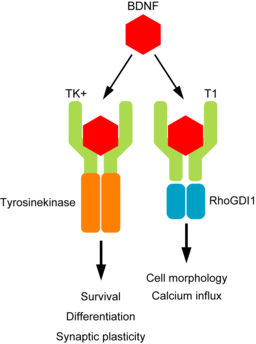
Brain Derived Neurotrophic factor (BDNF) protein is an important neurotrophin responsible for regulating many aspects of growth and development in different cells within the CNS. The NTRK2 gene encodes the TrkB protein, which is an important receptor that binds extracellular BDNF and propagates the intracellular signalling response via a tyrosine kinase.
The NTRK2 gene expresses a number of different transcript variants in different cell types. The most well studied of these is the full length TrkB receptor referred to as TrkB, which is mainly expressed in neuronal cell types. The other transcript variants all express the same exons encoding the extracellular domain of the receptor (shown in green in the figure below) but have truncated intracellular domains, which do not include the tyrosine kinase domain and thus activate different signalling pathways upon binding to BDNF. None of these truncated protein products have been well studied, but the most highly expressed receptor variant is known as TrkB-T1, and is known to be highly expressed in astrocytes.
Since the transcript variants are differently expressed in different cell types within the CNS, the NTRK2 gene is a very useful example for exploring cell type specific transcript expression in available public data.
Content from UCSC Genome Browser: Setup
Last updated on 2025-12-22 | Edit this page
Overview
Questions
- How do we navigate the web interface of the UCSC Genome Browser?
Objectives
- Become familiar with basic navigation and configuration of the UCSC Genome Browser
Navigating the UCSC browser
Many of the tools that we will explore in this section can be selected via multiple different routes within the browser interface:
- Many tools can be accessed via the top toolbar on a pull down list
- Other tools can be accessed from within the browser window
In the following instructions, we will mostly navigate through successive lower levels from the pull-down menu from the top toolbar. Code-style text indicates buttons to click or options to select from a pull-down menu, with successive instructions indicated by > . For example: the below indicates that you should select Genome Browser from the top tool bar and then click on Reset all user settings.
Toolbar > Genome Browser > Reset all user settings
The UCSC Genome Browser is supported by a rich training resource which has new material added regularly to the YouTube channel.
To access training and develop your skills further, go to:
Toolbar > Help > Training
WARNING
Weekly maintenance of the UCSC browser occurs at 2-3pm Sundays Pacific time (7-8am Mondays AEST / 8-9am Mondays AEDT). During this time the browser may be down for a few minutes.
To ensure uninterrupted browser services for your research during UCSC server maintenance and power outages, bookmark one of the mirror sites that replicates the UCSC Genome Browser.
More information and contacts for the UCSC Genome Browser can be found here.
Setting up your browser
1. Open the Browser interface
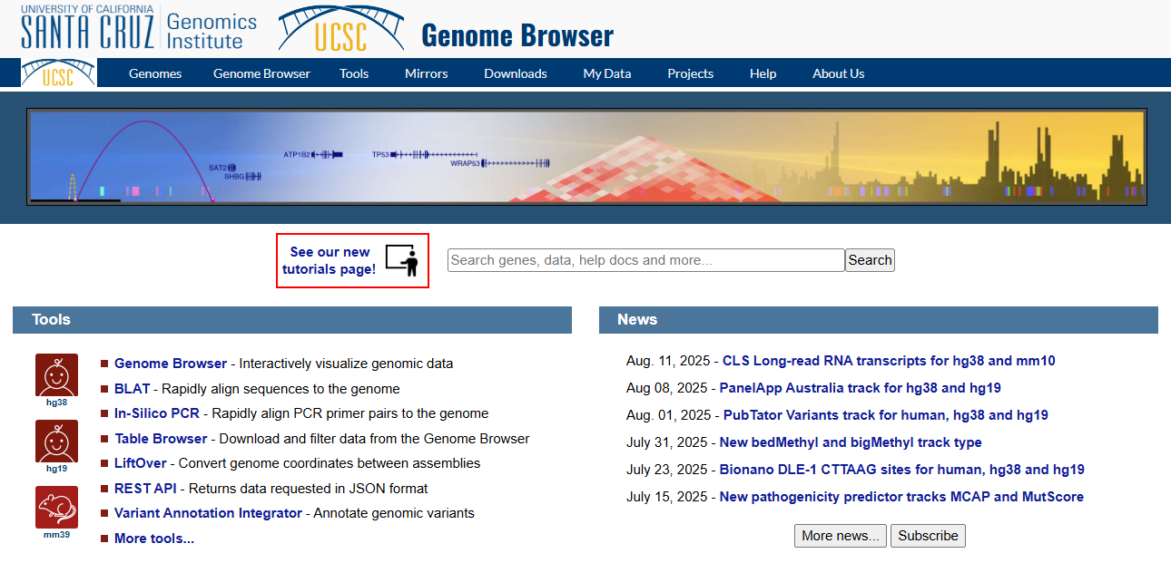
Navigate to the UCSC Genome Browser and sign in if you have an account.
2. Reset the browser
To ensure we all see the same screen, select:
Toolbar > Genome Browser > Reset all user settings
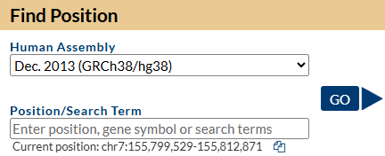
3. Select and open the human Genome Hg38 at the default position
Toolbar > Genomes
Ensure that GRCh38 is selected in ‘human assembly’ and click on the
blue GO box
You should see a view of the browser similar to the image below, opening at a position on chromosome 7 of Human genome version GRCh38 showing the gene model for the SHH gene. Some of the default tracks may have been updated since this screenshot was made.
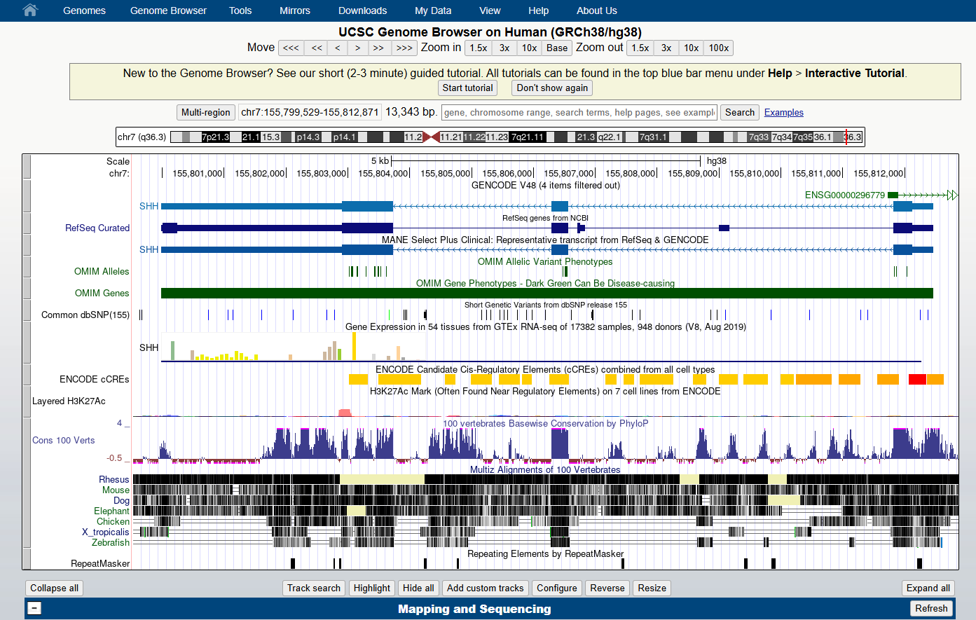
4. Familiarise yourself with the main areas of the interface
Can you locate:
- The main toolbar
- Blue bar track collections (data of similar types are collected together under the same ‘Blue bar’ heading). Scroll down to see additional data collections and which ones are turned on as default.
- Genome species and version number
- Position box
- Navigation tool buttons
- Chromosome ideogram
- Genome view window
- Pre loaded tracks, track titles:
- The grey bars on the left of the genome view can be used for selecting and configuring the tracks.
- You can change the order of the tracks by dragging these grey bars up and down.
- Turn tracks on and off:
- You can hide tracks by right clicking on the grey bar or by turning them off in the Blue bar collections.
- You have to click on a ‘refresh’ button for changes to be reflected in the genome view window.
- View the configuration page for one of the tracks.
The configuration page gives you a lot of information about the data
track and its colouring. You can open the configuration page for a track
by:
- clicking on the grey bar for the track or,
- clicking on the track title in the Blue bar collection. More information and options are usually available by selecting the configuration page for a track via the track title in the Blue Bar collections.
- Select the
resizebutton under the genome view to fit the genome view window to your screen
6. Practise navigating around the genome view
Can you practise:
- Moving left and right, using both the navigation buttons and your mouse
- Zooming in and out, using navigation buttons
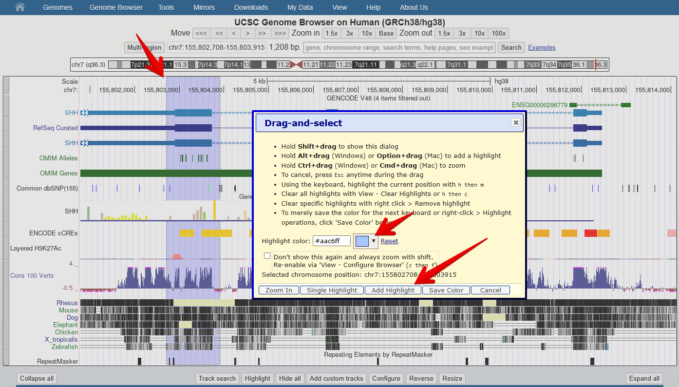
- Zooming in to a region of interest, using
drag-and-select:- Using your mouse, select a region of interest by clicking the ruler (position track) at the very top of the genome view window. Hold down the left click and drag to select a larger region.
- This is also how to access the highlight tool which
you will use in a later exercise to highlight a region of interest.
- Click on the down arrow next to the highlight colour to select a different colour.
- Don’t forget to click
Add Highlightto save your highlighted region on the genome
- The UCSC genome browser can be easily configured according to your visual preferences and data needs
Content from UCSC Genome Browser: Understanding gene models
Last updated on 2025-12-22 | Edit this page
Overview
Questions
- How do we interpret gene models represented in the UCSC genome browser?
Objectives
- Understand how genomic data is represented in the UCSC genome browser
- Identify differences between transcript variants
Now we will explore some tools and public datasets available in the UCSC genome browser.
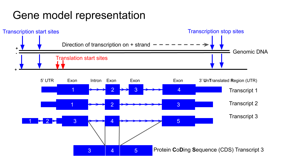
Gene model representation
NTRK2
First we are going to familiarise ourselves with the gene model representation of the different transcripts of NTRK2.
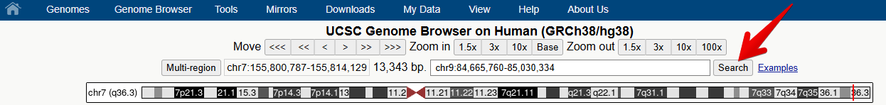
1. Navigate to the NTRK2 gene position in GRCh38 and view the gene models.
You can navigate to a different region of the genome by typing in the position box.
If you know the specific location you are interested in, type in the location (e.g. chr9:84,665,760-85,030,334)
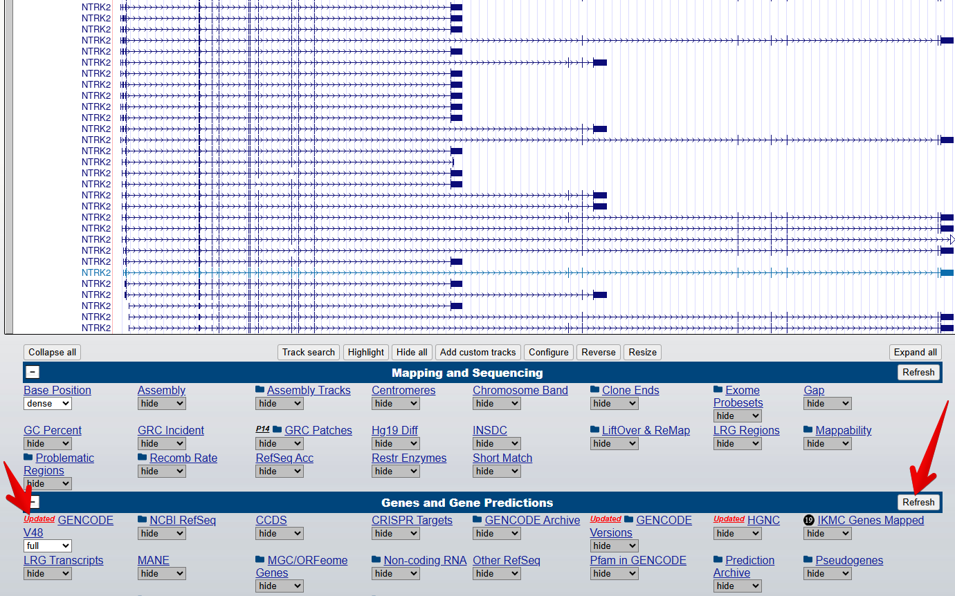
3. Turn on the Gencode track
From the blue bar group labelled
Genes and Gene predictions, set GENCODE V48 to
full and select Refresh to turn on the gene
modelling track. Note: the version number 48 may have changed since
this workshop was last updated.
4. Turn on the Conservation track
From the blue bar group labelled Comparative Genomics,
set UCSC 100 Vertebrates to full and select
Refresh to turn on the conservation track.
5. Zoom out and scroll across the whole gene
Zoom out until you can view all of the 5’ UTRs and 3’ UTRs for all
transcript variants for this gene. Then drag the view left and right to
centre the transcripts or use drag-and-select to
Zoom In.
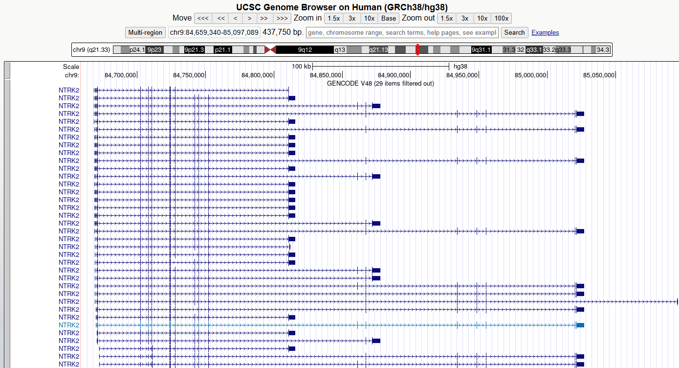
CHALLENGE 1
Which strand is the gene encoded on / transcribed from? (+ or - strand)
The positive (+) strand. We know this because we can see the right-facing arrow ticks in the intronic regions of the gene model.
CHALLENGE 2
Identify the exons, introns and UTRs.
Do regions of conservation only occur were there are coding regions?
Compare the NTRK2 transcript tracks to the gene model representation at the top of this lesson and discuss with your neighbour to identify exons, introns and UTRs.
Peaks in the conservation track indicate regions of high conservation
across species. Use drag-and-select to zoom in to some
non-exonic regions of high conservation (you may need to drag and select
multiple times to zoom in far enough).
CHALLENGE 3
How many different transcripts variants are there for this gene?
How do they differ?
Count the number of items in the GENCODE track. Hover over each
transcript to view its ID. You may also wish to turn on the
NCBI RefSeq track to view the NCBI RefSeq transcript
IDs.
Notice how the number and position of exons, introns, and gene length differ between transcripts.
CHALLENGE 4
Select a coding region/exon towards the 3’UTR of the gene. Zoom in to the region until you can see the letters of the amino acid sequence. Then do the same for a coding region/exon towards the end of the 5’UTR of the gene.
Why are some amino acid boxes red or green?
Green boxes indicate potential start codons, red boxes indicate translation termination codons.
CHALLENGE 5
Zoom in further until you can see each amino acid number.
Why do different transcripts have different amino acid numbers?
Different transcripts may have different exons, or exons of different lengths, so as you move further towards the end of the gene, the amino acid numbers between different transcripts may no longer match.
NOTE
Note that one of the transcript names is highlighted in a different colour: this is the transcript you selected from the autocompleted list or the search results.
6. Change the view settings for the track
Right click on the track grey bar in the left of the genome window to access view settings.
Switch between dense , squish ,
pack , and full to see how it changes the
representation of the models.
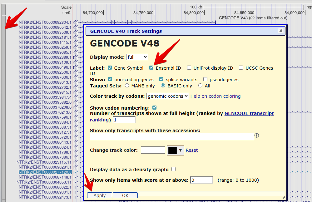
7. Reveal the Ensembl ID for each transcript
Right click on the GENCODE track grey bar and select
Configure GENCODE v48to go to the configuration page.Check the box to also reveal the
Ensembl IDin the label.Select
Applyto save your changes.
The transcript names are now too long to fit on the screen. You can
use the configuration page (like you did to change the font size
earlier) to change the number of characters in the
Label area width so that you can see the entire transcript
label.
Check your understanding
Question 1
Which transcript encodes the shortest amino acid sequence?
ENST00000352327.5
This transcript does not include one of the large coding regions and the coding region in the terminal exon is also slightly shorter.
Question 2
Which transcript has the longest 3’UTR?
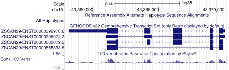
ENST00000396976.6
Although the last two exons of ENST00000396972.2 are UTR rather than coding sequence, it is still not as long as the 3’UTR of ENST00000396976.6
Question 3
Which transcripts appear to encode the same protein product?
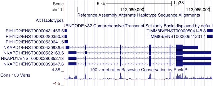
ENST00000420986.6, ENST00000280352.13 and ENST00000393047.8
Notice the height of the boxes for the first three exons: ENST00000532163.5 appears to encode a different CDS from the other transcripts.
Question 4
Which transcript has the longest 5’UTR?
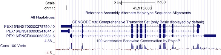
ENST00000532681.5
This transcript is encoded on the reverse strand.
Question 5
Which transcript has the longest CDS?
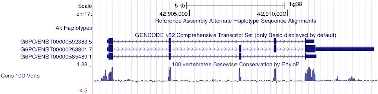
ENST00000253801.7
This transcript is encoded on the forward strand.
Question 6
Which transcript has the longest 5’UTR?
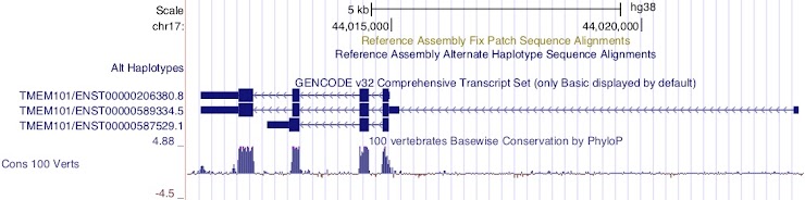
ENST00000589334.5
This transcript is encoded on the reverse strand.
BDNF
Now we will look at the gene model for BDNF in the same genome. There are some differences that enable us to demonstrate some more tools.
1. Navigate to the BDNF gene position in GRCh38
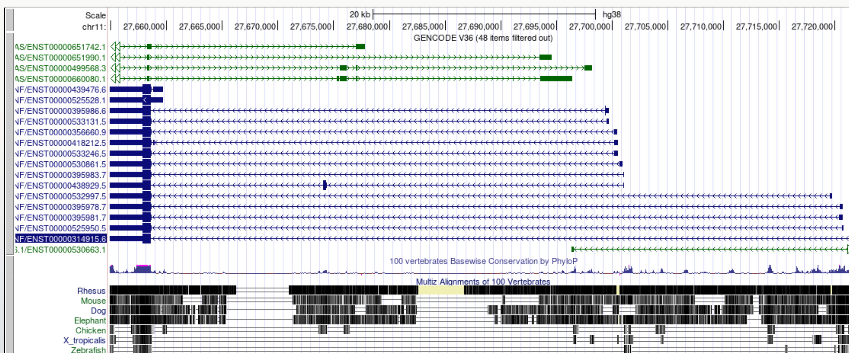
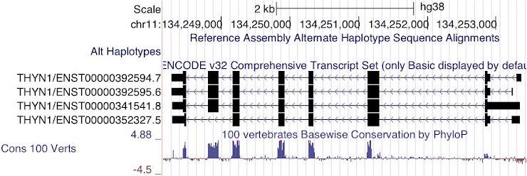
- Note that there are blue transcript models encoded on the - strand and green BDNS-AS transcript models on the + strand. BDNF-AS is the antisense gene.
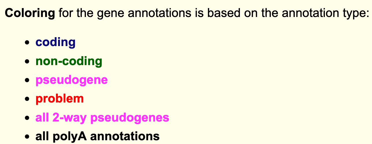
- Colouring information is specific for each track and can be obtained from the configuration page. Below is the colouring legend for the GENCODE V36 track.
2. Flip the orientation of the gene
Since the convention is to display genes in the 5’ to 3’ orientation, it can be useful for our own interpretation, and also for presentation purposes, to flip the orientation of a gene when viewing it in a Genome Browser.
To flip the orientation of the gene, use the reverse
button under the genome view window.
3. Apply the Multi-Region view from the main tool bar view options
When a gene has many large introns taking up a lot of white space in an image, it can be difficult to see if exons in different transcript models or other data tracks align. The Multi-Region view tool can be used to fold the intronic regions out of the view like a concertina. The Broswer selects which region to fold out based on the gene model track(s) that you have turned on at the time.
Toolbar > View > Multi-Region > Show exons using GENCODE V48 > Submit
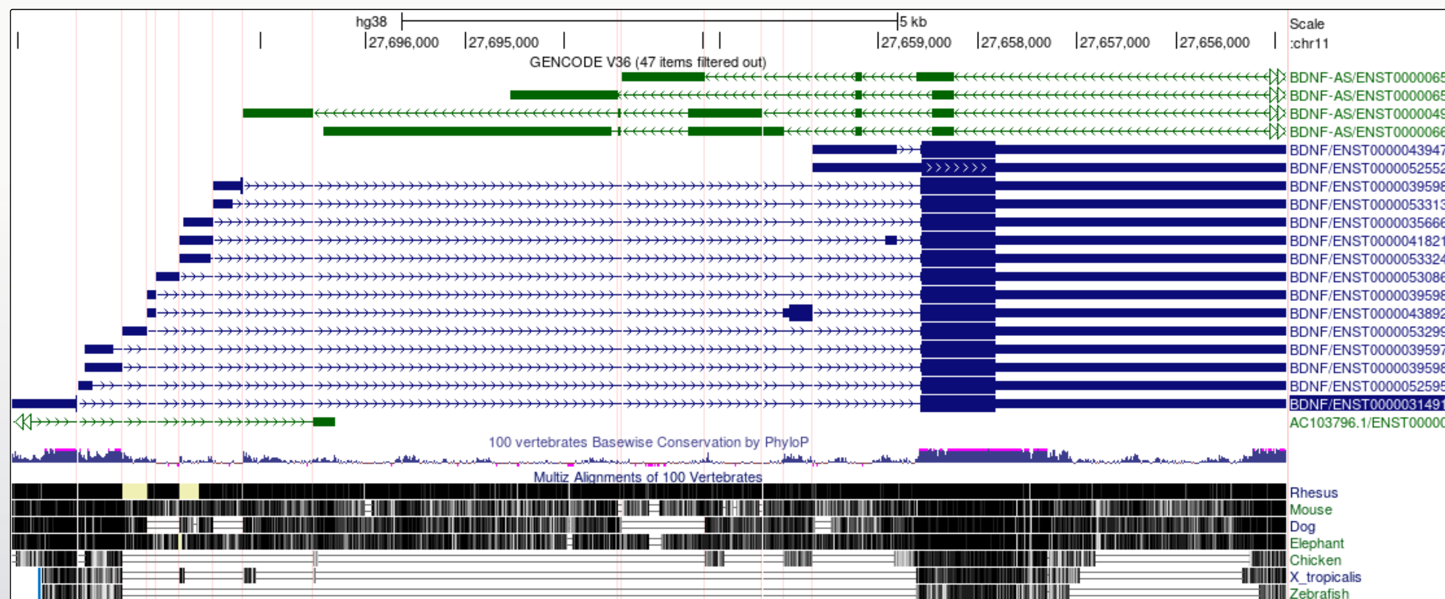
Did you notice?
- The transcript variants for the BDNF gene vary mostly in the genomic position of the 5’UTR.
- The noncoding BDNF-AS gene transcript includes a region that would be antisense to the coding BDNF transcript.
You may find that using the multi-region tool facilitates visualisation and interpretation of gene expression data later in the workshop.
- The UCSC genome browser graphically represents key elements of gene transcripts, including exons, introns, and untranslated regions
- Different settings and tools can be used to configure the browser to more easily investigate specific features of a gene.
Content from UCSC Genome Browser: BLAT tool
Last updated on 2025-12-22 | Edit this page
Overview
Questions
- What is the BLAT tool and how do we use it?
Objectives
- Use the BLAT tool to locate genomic regions with similarity to a sequence of interest
The BLAT tool
The BLAT tool is a sequence similarity tool similar to BLAST. It can quickly identify region(s) of homology between a genome and a sequence of interest. Due to the presence of orthologs and paralogs, a target sequence may have similarity to more than one region in the genome.
Exercise
In this exercise, we will employ the BLAT tool to map the sequences of two different expression probes to their target regions and determine which NTRK2 gene transcripts the probes are likely to detect.
A note on microarray expression data
Microarray expression data is not commonly used now, but some of the data generated from large, well-orchestrated studies still provide valuable information to researchers. Microarray probes, like in situ hybridisation probes, target a small region of the RNA and do not measure the whole RNA transcript. If you are measuring gene expression, it is important to know exactly which region of the gene you are detecting.
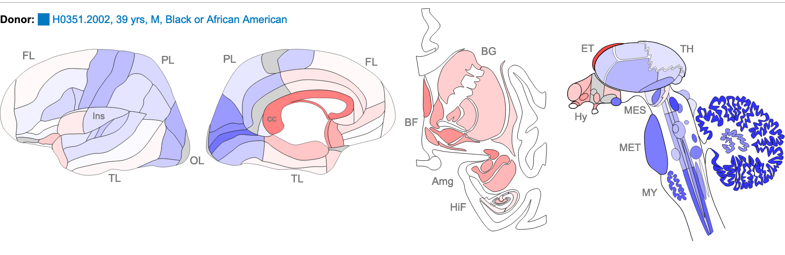
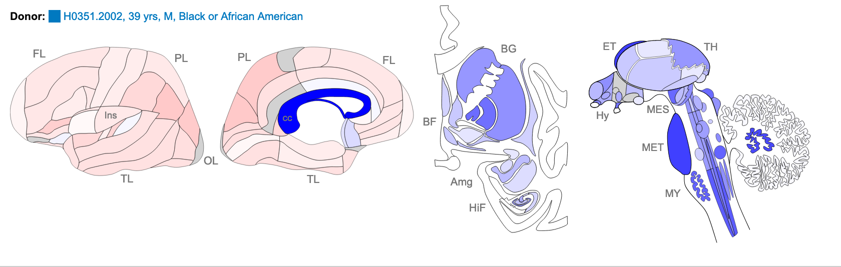
The study was the Human Brain Gene Expression Atlas generated by the Allen Institute. Below are sequences of two hybridisation probes that were use in a microarray used to detect expression of the NTRK2 gene. These two probes result in very different hybridisation and expression patterns across different regions of the brain. As we observed in the previous exercise, NTRK2 has a number of different transcript variants.
Our question: are these probes detecting different NTRK2 transcripts, and if yes, which ones?
The probes
The images below are of one of the six donors included in the atlas, and typical of the expression pattern for NTRK2. These images are taken from the NTRK2 gene page of Human Brain Atlas.
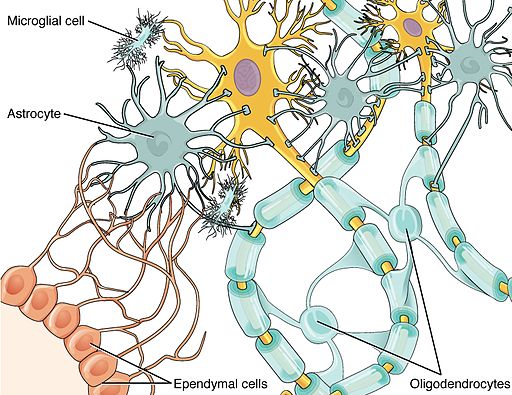
Most obvious in the images is the high level of expression signal using Probe A_23_P216779 and low level for A_24_P343559 in the corpus callosum (CC), which is a region of white matter in the brain with relatively few neurons and relatively high proportion of myelinating oligodendrocytes. This expression profile is reversed in the the cortical regions, eg. frontal lobe (FL) and parietal lobe (PL), which have a relatively high density of neuronal cells.
Your task
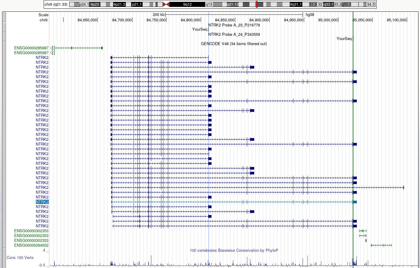
1. Use the BLAT tool to find region of homology
Select
Toolbar > tools > blatCopy the sequence of the first probe above and paste into the search box
Under
Assembly, select the human GRCh38 and clickSubmit

Select
Rename Custom Track. Copy and paste the probe name to use as the label for theCustom track nameandCustom track description. ClickSubmit. It is not necessary to build a custom track, but this enables you to give your sequence a unique name which is important if you are doing multiple BLAT searches and want be able to tell which one is which.Select
browserfor the hit with the highest homology to view the result. Observe which region of the NTRK2 gene this probe will target. Zoom out for context.Note that a new blue bar heading has appeared for your custom tracks.
Repeat for the other probe sequence.
2. Use the highlight tool to keep track of region of interest in the genome view.
It is easy to lose track of a region you are investigating when navigating around the genome in a browser. We are going to highlight each region of probe homology within the NTRK2 gene, using a different colour for each probe. Highlight is also useful if you have lots of different tracks loaded and you want to check that a feature on one track lines up with another.
Use
drag-and-selectto select only the region of homology for each probe within the NTRK2 gene. Use a different highlight for each region.Zoom out to view the whole gene again.
DISCUSS
Do the probes detect coding regions of the NTRK2 gene?
Discuss
Are the probes likely to detect different transcripts?
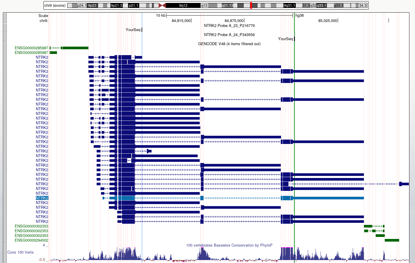
3. Use ‘Multiregion view’ to make it easier to compare coding regions of different transcripts
Toolbar > View > Multi-RegionSelect
Show exons using GENCODE V48
- We can use the UCSC BLAT tool to identify region(s) of similarity between a sequence of interest and other parts of the genome.
Content from UCSC Genome Browser: Gene expression data
Last updated on 2025-12-22 | Edit this page
Overview
Questions
- How can we explore gene expression data in the UCSC genome browser?
Objectives
Use the UCSC gene browser to:
- Compare a region of one genome to genomes of other species
- Determine the tissue/cell type expression profiles of a gene of interest in mouse and human expression data
Viewing GTEx data in the UCSC Genome Browser
Human tissue specific expression data from the GTEX project is available in the UCSC genome browser.
Gene level expression data from
GTEx Gene V8donors can be turned on from the blue bar underExpression. These are displayed as coloured bar plots.Transcript level expression data is available by turning on
GTEx Transcriptunder the same blue bar. This is also displayed as bar plots.-
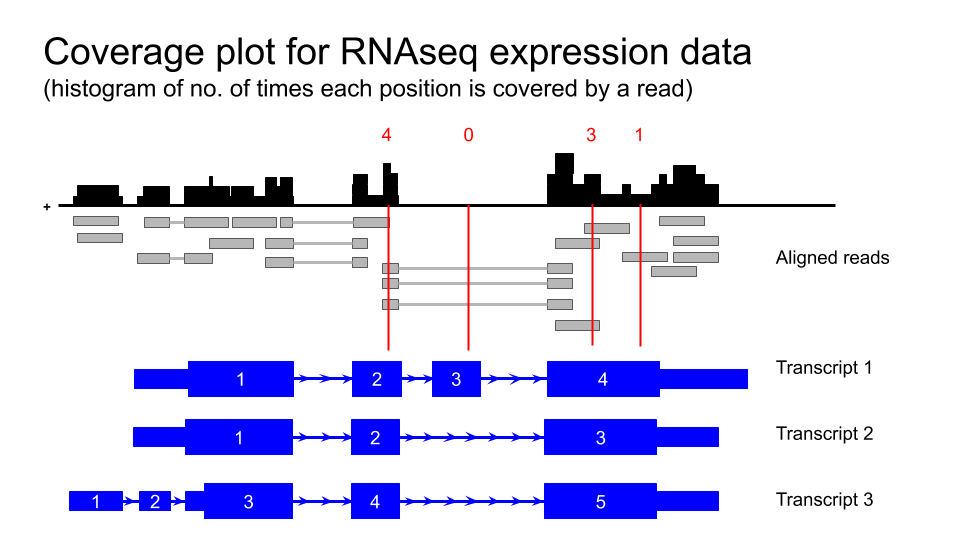
Transcript level expression data for GTEx V6 is also available as coverage plots.
Toolbar > My data > Track Hubs- Scroll down to
GTEx RNA-seq Signal Hub. Selecthg38

Default settings
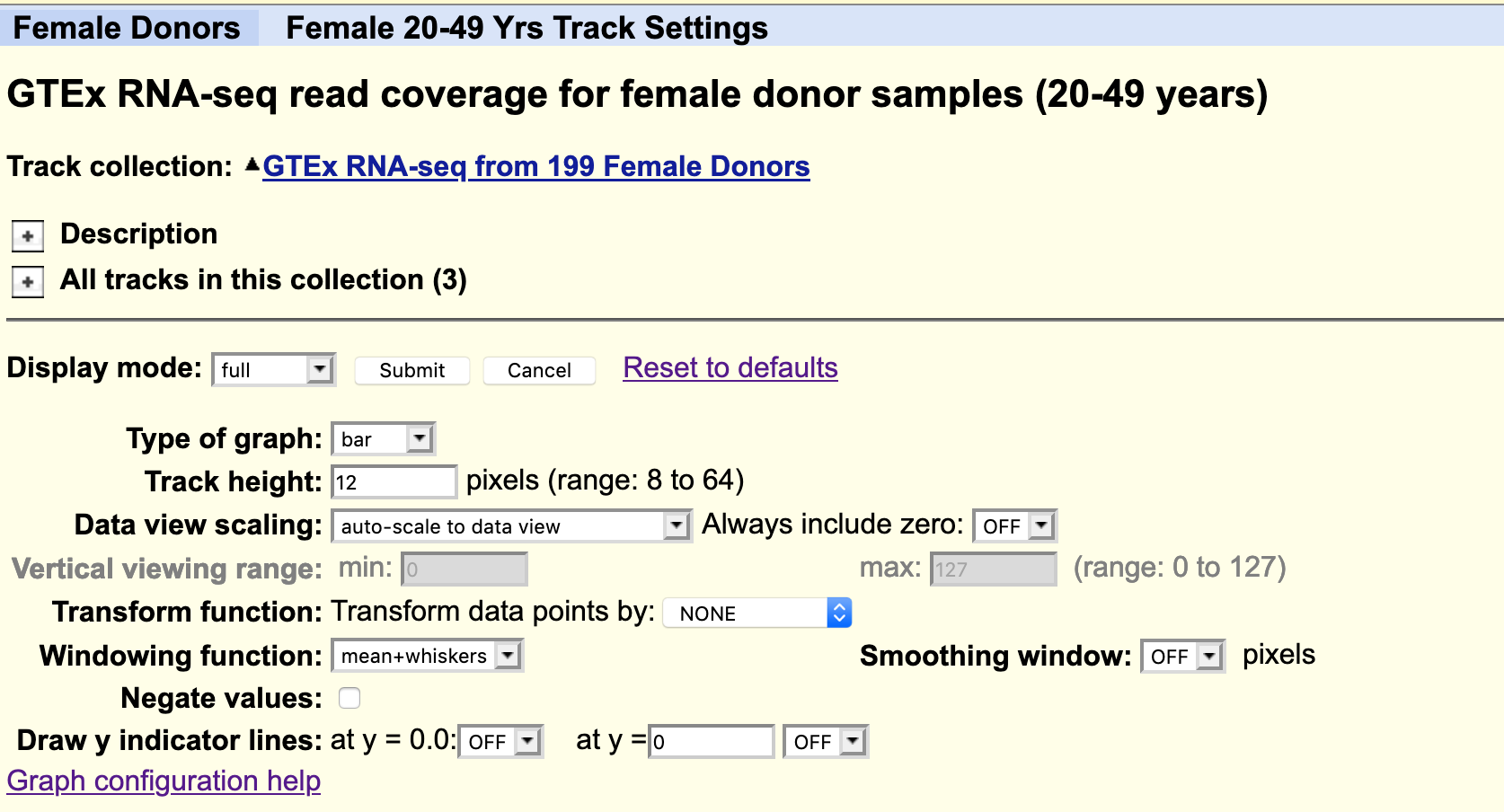
By default, all the available data from one individual only is loaded. Data from other subjects in the study can be loaded as desired. For example, you could load all available samples for one tissue region only.
The data is autoscale to data view with a track height or 12 pixels for each samples. You can change the height of the track or add a data transformation.
As usual, you can right click on the grey bar on the left hand side to configure the track set.
Your task
Using the selection matrix for female donors aged 20-49 years, deselect the default samples and select only Brain cortex and Pancreas samples.
Navigate to the location for the gene MYRF. You can increase the height of the datatrack to improve visualisation.
CHALLENGE 1
Can you locate an exon in the MYRF gene that is present in transcripts expressed in the brain but not in the pancreas?
CHALLENGE 2
Does this alternative splicing event result in a frame shift of the coding sequence?
CHALLENGE 3
How many amino acids are there in the protein products for each MYRF transcript?
FACS data
The FACS derived data from the Tabula Muris cell type data can be visualised as a coverage plot.
Your task
Navigate back to the NTRK2 gene in the human genome. Navigate to the Ntrk2 gene in the mouse genome via
Toolbar > View > In Other Genomes (Convert)Under
New GenomeselectMouse, underNew AssemblyselectGRC38/mm10, then clickSubmitSelect the region with the greatest homology
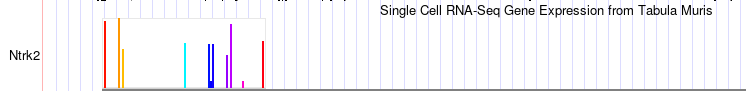
Click on the bar chart icon for the Tabula muris data in the default view to see a summary bar chart of the cell type data.
- To see a coverage plot of the expression data, we have to configure
the Tabula Muris track.
- Right click on the grey bar to
Configure Tabula Muris track set - Hide
Cell expression - Select
Genome coverageto full - Select
submit
- Right click on the grey bar to
This can look a bit overwhelming as there are many tracks and the default track height is set very high, but it is easy to simplify it by focusing on a few cell types of interest.
- Right click on the grey bar to
configure Genome Coverage track set- Change
Track heightto 30 pixels - for
Data view scalingselectgroup auto-scale -
Hide Allsubtracks and then manually select only these few cell types of interest:- astrocyte Cv
- Bergmann glial Cv
- microglia Cv
- neuron Cv
- oligodendrocyte Cv
- OPC Cv
Submit
- Change
CHALLENGE 4
Which cell type has the highest level expression of Ntrk2 in this dataset?
Go back to the configuration page to change
Data view scalingtoauto-scale to data viewandSubmitExport a PDF image of the genome view:
Toolbar > View > PDFselectDownload the current browser graphic in PDF
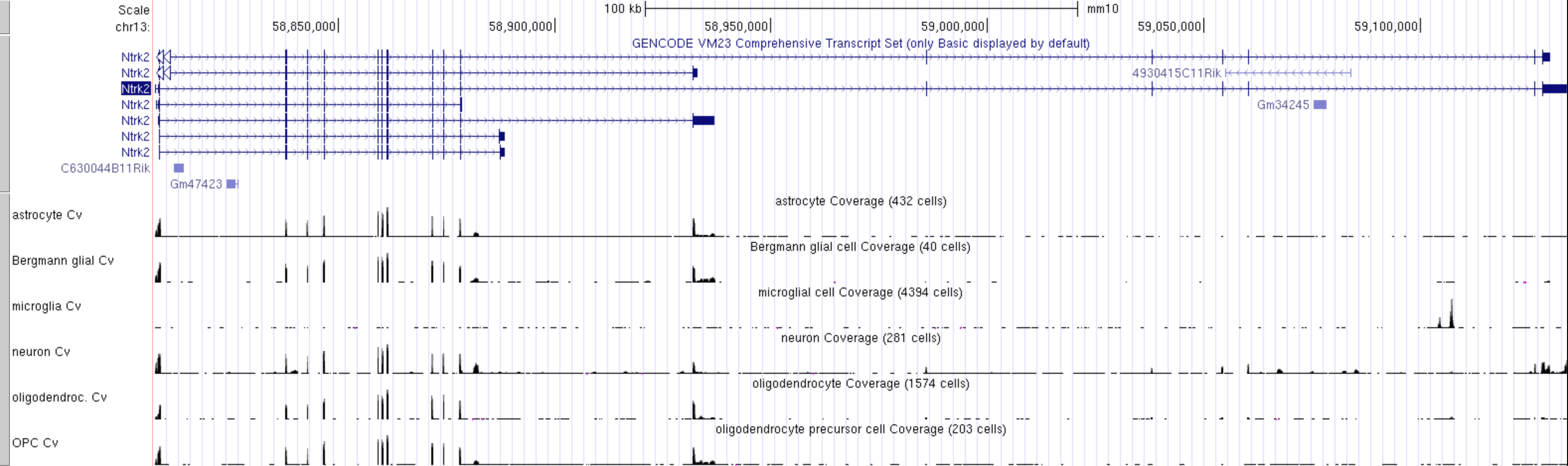
CHALLENGE 5
Which cell type(s) express the long and short transcripts of Ntrk2?
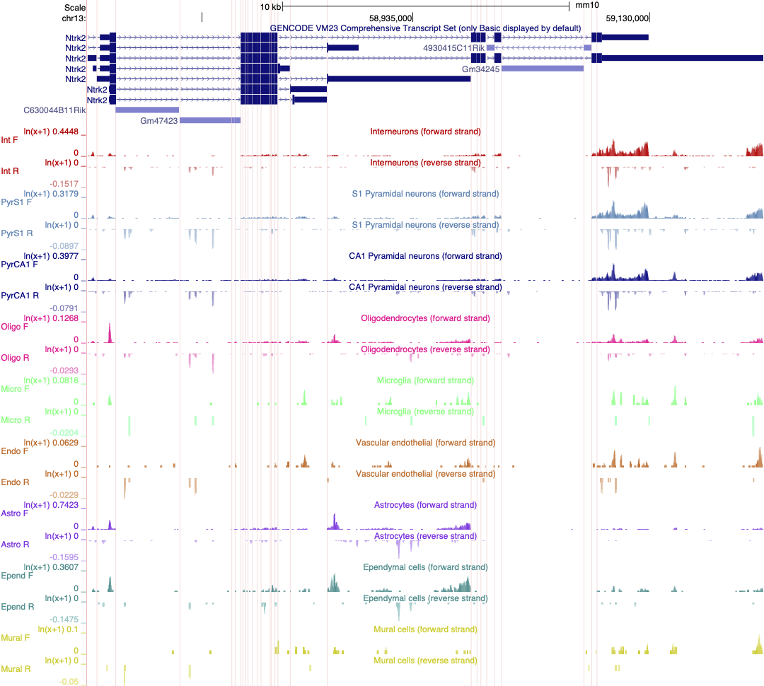
Linnarsson lab data
Mouse CNS cell type expression data can also be validated using an independent single cell dataset of mouse cortex from the Linnarsson lab.
The data that is publicly available for viewing in the UCCS genome browser is not housed in the UCSC genome browser. You must first access it from the the Linnarsson lab data page.
This RNAseq data is stranded, meaning you can see if the transcript data is from the + or - strand.
Your task
Click here for the Linnarsson lab public data page for this dataset where you can search for cell expression profiles for individual genes.
-
Click on the
Browse the genomeblue text near the bottom of the page.This loads 18 different tracks, one for each cell type investigated. The default setting for expression range is quite high and most gene expression is not observed with these settings. Each track must be configured individually rather than as a group, which takes a lot of time.
We previously created a version of this data where each track is autoscaled which can make it quicker to determine which expression range would be ideal for visualising the expression of an individual gene. The session is illustrated in the screen shot below. Note that the data is also viewed using ‘Multi-Region’ which hides the introns in the gene models.
CHALLENGE 6
Select two or three cell types in your session and adjust the scale to best reflect differences in gene expression of Ntrk2 between these cells.
Save this session and share it.
- The UCSC genome browser allows you to compare gene expression data from multiple different sources and species
Content from IGV
Last updated on 2025-12-22 | Edit this page
Overview
Questions
- How do you use IGV?
Objectives
- Learn how to open basic file types and navigate IGV
- Understand the type of data that can be visualised in IGV
IGV
In this section we will download a BAM file of gene expression data from SRA, and view it in the Integrated Genome Viewer (IGV). BAM files must first be sorted and indexed before they can be loaded into genome viewers. IGV has tools to do this without having to use the command line.
Exercise
The data
The expression data we are using for this exercise is from the mouse Celltax single cell expression atlas published by the Allen Brain Institute. The cell tax vignette has an expression browser that displays gene level expression as a heat map for any gene of interest. The readsets (fastq files) and aligned data (BAM files) for 1809 runs on single cells are also available for download from SRA.
The SRA study ID for this study is SRP061902 and individual runs from this study are easily selected by viewing the samples in the ‘RunSelector’.
For this exercise, we will download a few samples in order to illustrate navigating in IGV by looking at the expression of NTRK2 in the same cell types we have discussed in earlier exercises. For each cell type, we will down load a .BAM file containing only the reads from the chromosome of interest.
Your task
1. Download BAM files from SRA
For each SRA run in the table below:
Click on the SRA run to open the link.
Click on the ‘Alignment’ tab. Note that the data is aligned to the mouse GRCm38 genome (mm10).
Select the chromosome of interest. For Ntrk2 in mouse it is chr13
For
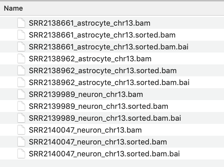
Output this run in:selectBAMand click onformat to: FileRename the downloaded file to include the cell type, to avoid confusion, e.g. SRR2138661_astrocyte_chr13.bam
| Cell type | SRA run | Vignette Cell ID |
|---|---|---|
| astrocyte | SRR2138962 | D1319_V |
| astrocyte | SRR2139935 | A1643_VL |
| neuron | SRR2139989 | S467_V4 |
| neuron | SRR2140047 | S1282_V |
2. Use IGV tools to SORT and INDEX the BAM files
Open IGV and select
Tools > Run igvtoolsfrom the pull down menusSelect
Sortfrom the Command options and use the browse options to select the BAM file you just downloaded. ClickRunWithout closing the igvtools window, now select the command
Indexand browse to find the BAM file you just sorted. It will have the same file name with ‘sorted’ added to the end, e.g. SRR2138661_astrocyte_chr13.sorted.bam
The resulting index file will have the file name SRR2138661_astrocyte_chr13.sorted.bam.bai
IMPORTANT
It is essential that the index file for a BAM file has the same name and is located in the same folder as its BAM file. If not, the IGV software will not be able to open the BAM file.
3. View the BAM files in IGV
Select the Mouse (mm10) genome from the genome box in the top right hand corner.
Select
File > Load from Fileand select all four _chr13.sorted.bam files only.Select
open- but don’t expect to see any data yet. The genome view window opens on a whole chromosome view as default but it wont show any data until the view region is small enough to show all data in the current view.Type the gene name NTRK2 into the search window.
Expand the Refseq gene model track by right clicking it to see all the splice variants.
-
The gene and thus the genome view is 328kb and the default setting for viewing data is only 100kb. Unless you have already changed your settings, alignment data will not get be showing. Zoom into the region of a coding exon by selecting in the numbered location track at the top of the genome view.
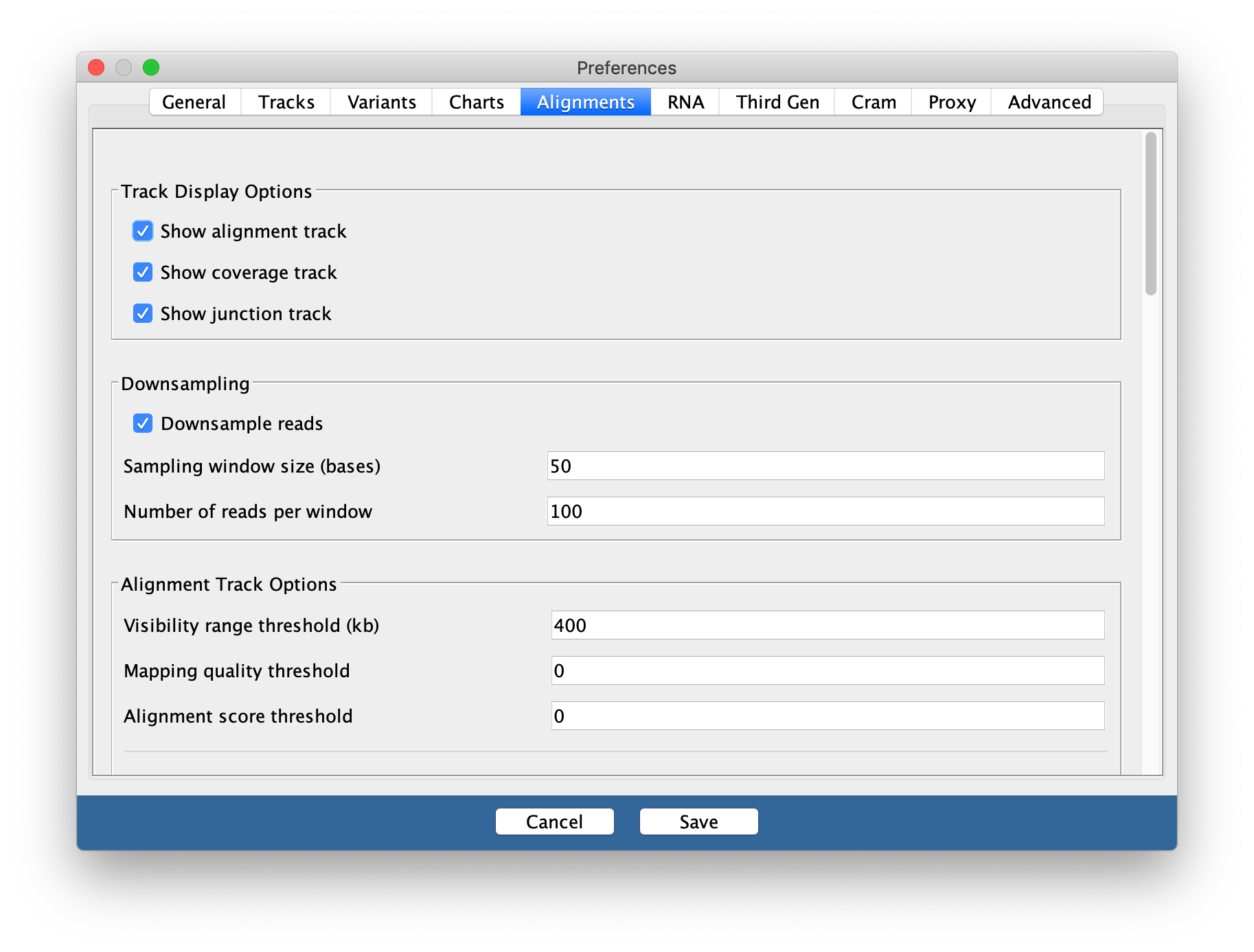
To see the whole gene in the genome window at the same time you may need to change the preferences.
Go to
View > Preferencesand select theAlignments tab. Change the visibility range threshold to 400kb.
4. Export images
The Genome view above can be exported by selecting
File > Save imagefrom the tool bar-
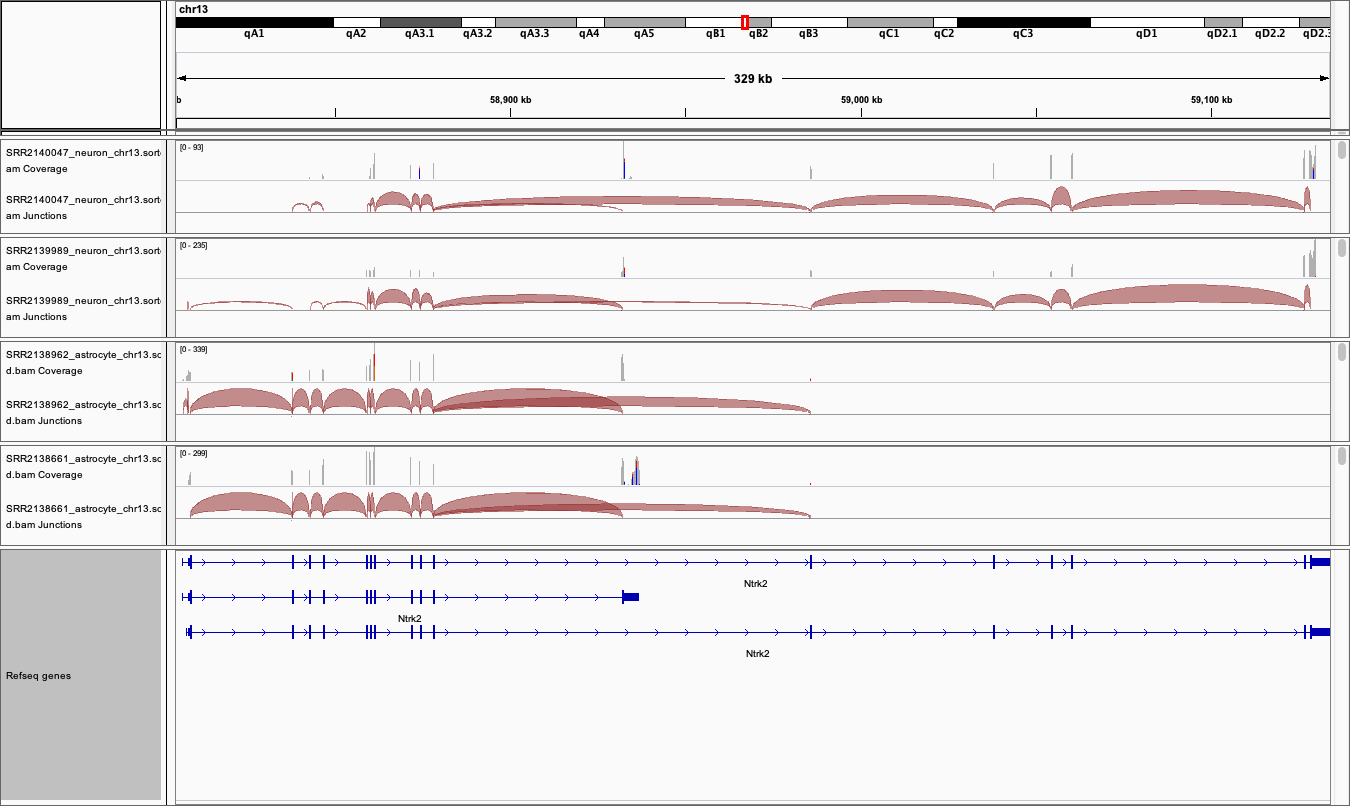
To export the Sashimi plot below:
- Right click on one of the junction tracks and select
Sashimi Plotfrom the pull down menu. - Select the tracks you want in your final image.
- There are some data filtering and style adjustments you can make to the Sashimi plot. Right click on each track to access the menu options. Some changes apply to each track individually and some to all tracks.
- Right click on one of the junction tracks and select
5. Download and install the Gencode gene model annotation track
The refseq gene model track is not as comprehensive as GenCode gene models. For both Human and Mouse the Gencode gene model gtf annotation files can be downloaded from Gencode. If you wish to do this be aware that it takes a little time and is not done as part of a workshop.
Create a folder called ‘annotations/Mouse’ in the main ‘igv’ folder that was installed on your computer when you downloaded IGV.
Download the GTF file from the link above and save it in this folder.
Unpack and then sort and index the .gtf file using igvtools.
In IGV, before you load you data files, load this annotation file and it will replace the refseq one.
If you would like to learn more about how to use IGV, please go to:
https://rockefelleruniversity.github.io/IGV_course/presentations/singlepage/IGV.html
- IGV can sort and index BAM files without use of the command line
- Sorted and indexed BAM files can then be opened to view genomic sequencing and gene expression data in IGV