All Images
Introduction to genome browsers
Data used in this workshop
Figure 1
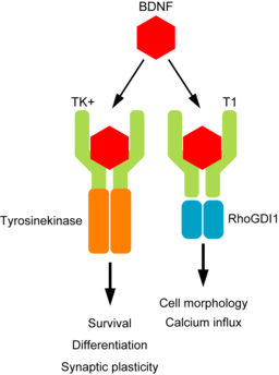
Graphical representation of the BDNF and TrkB
signalling pathway
Figure 2
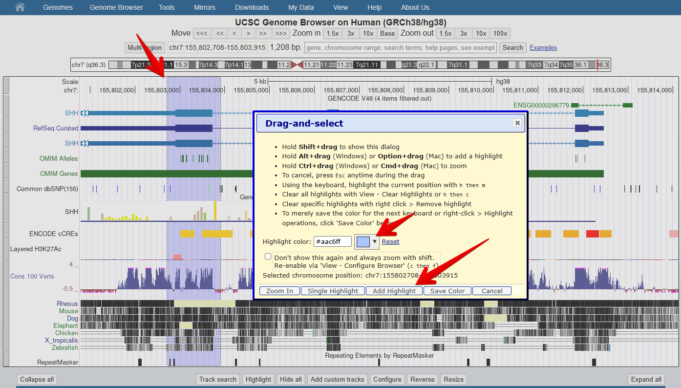
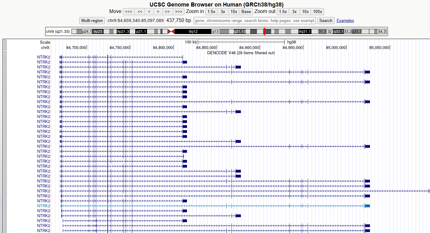
UCSC Genome Browser: Setup
Figure 1
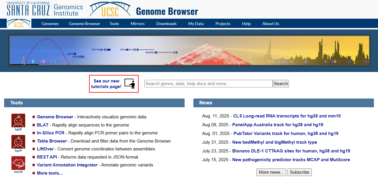
Figure 2
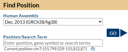
Figure 3
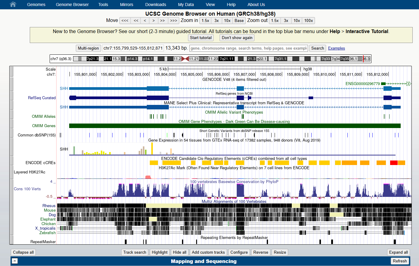
Figure 4
UCSC Genome Browser: Understanding gene models
Figure 1
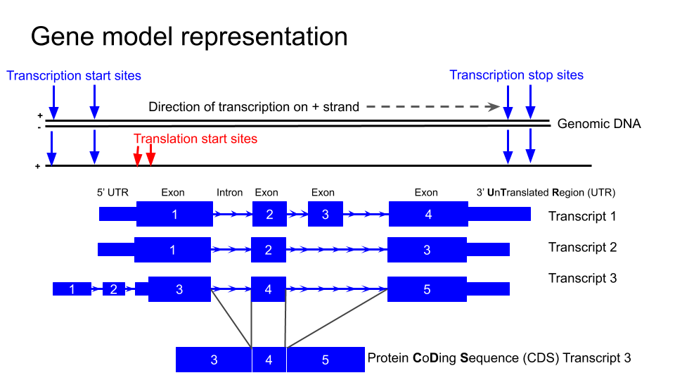
The typical structure of a gene as represented
in the UCSC genome browser
Figure 2
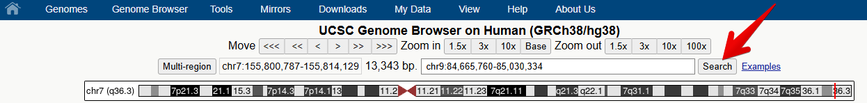
Figure 3
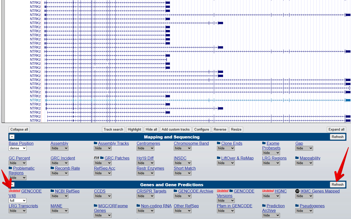
Figure 4
You should now see something like this
Figure 5
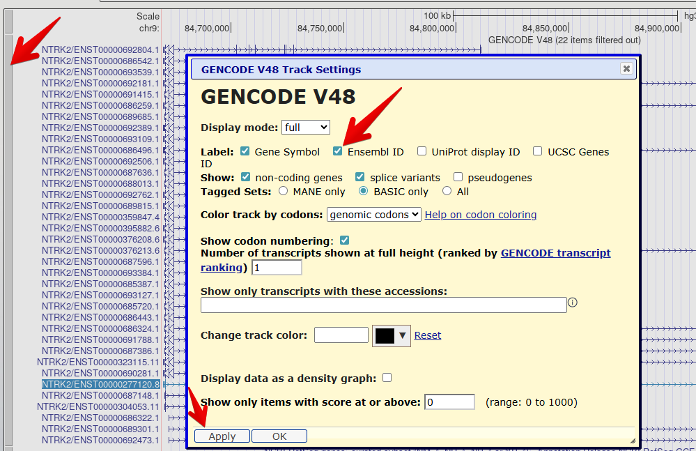
Figure 6
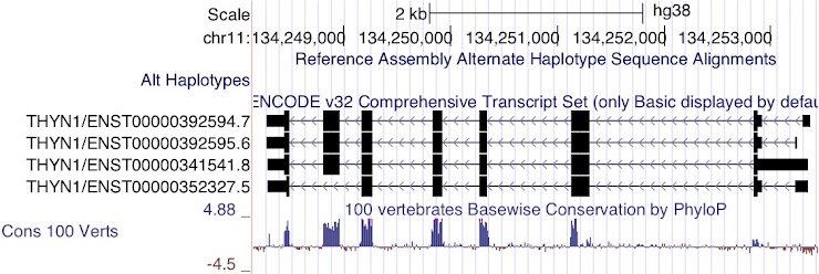
Figure 7
Figure 8
Figure 9
Figure 10
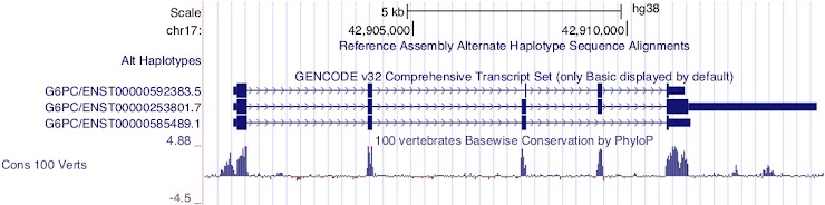
Figure 11
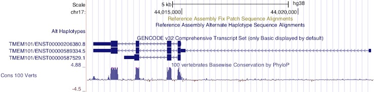
Figure 12
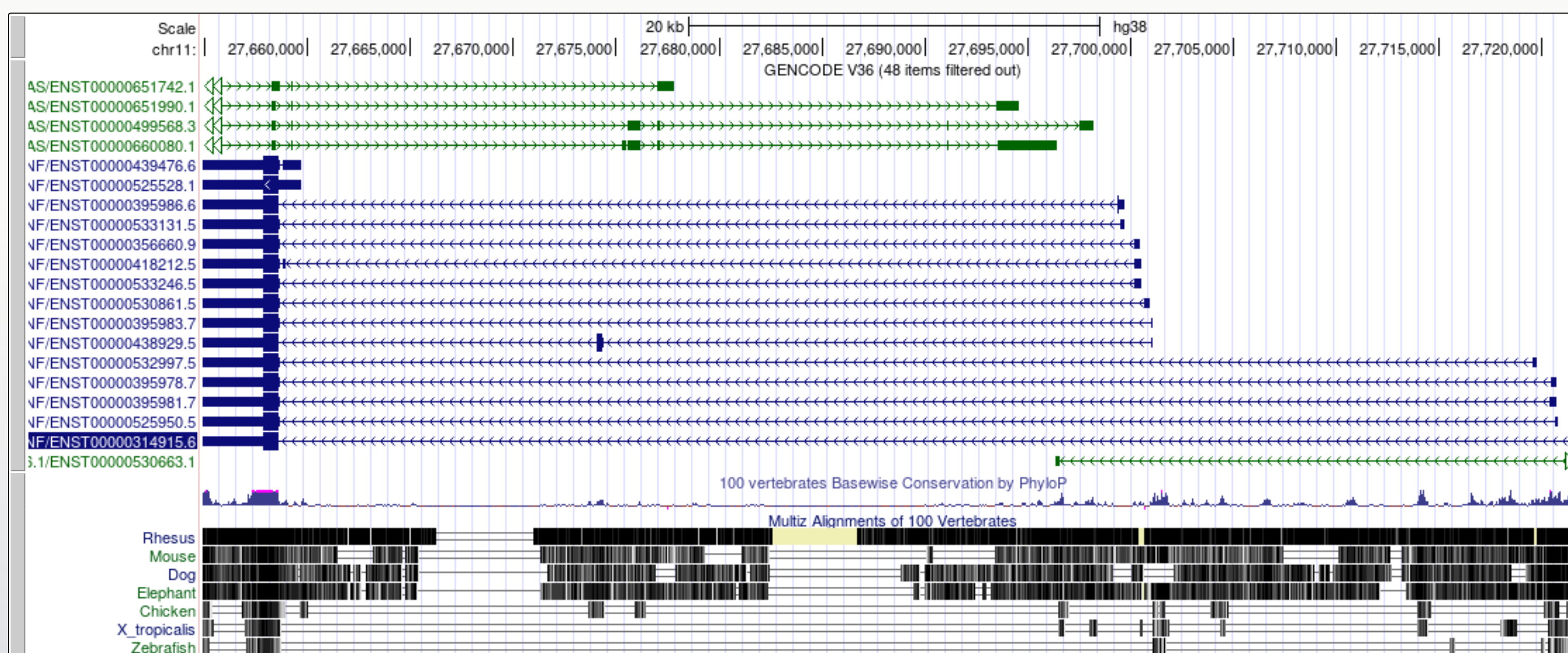
Figure 13
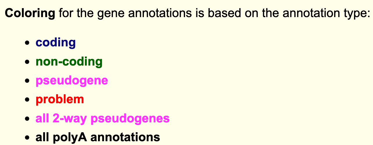
Figure 14
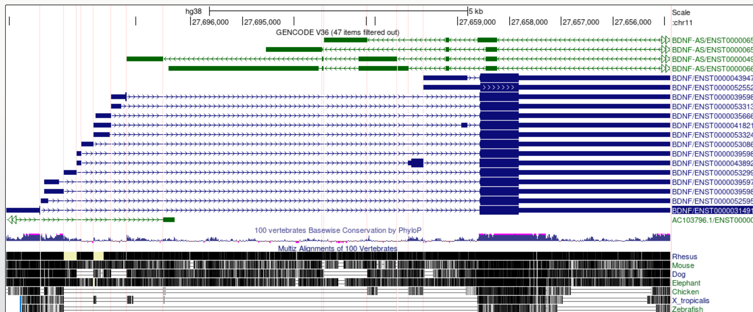
It is now a lot easier to view a number of
interesting features in the BDNF transcript models
UCSC Genome Browser: BLAT tool
Figure 1
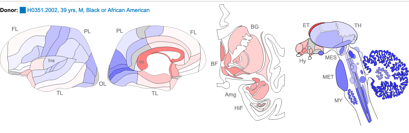
Z score of expression level in Human brain (blue
= low expression, red = high expression)
Figure 2
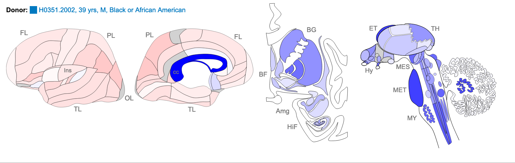
Z score of expression level in Human brain (blue
= low expression, red = high expression)
Figure 3

Probe A_23_P216779 returns 2 hits for different
chromosomes. One of these has 100% homology over the whole 60 base
sequence, the other has 87% homology over a 24 base region.
Figure 4
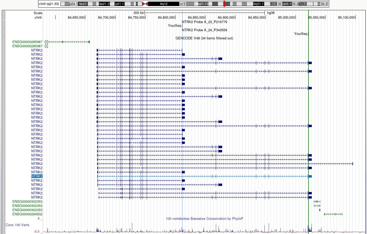
Figure 5
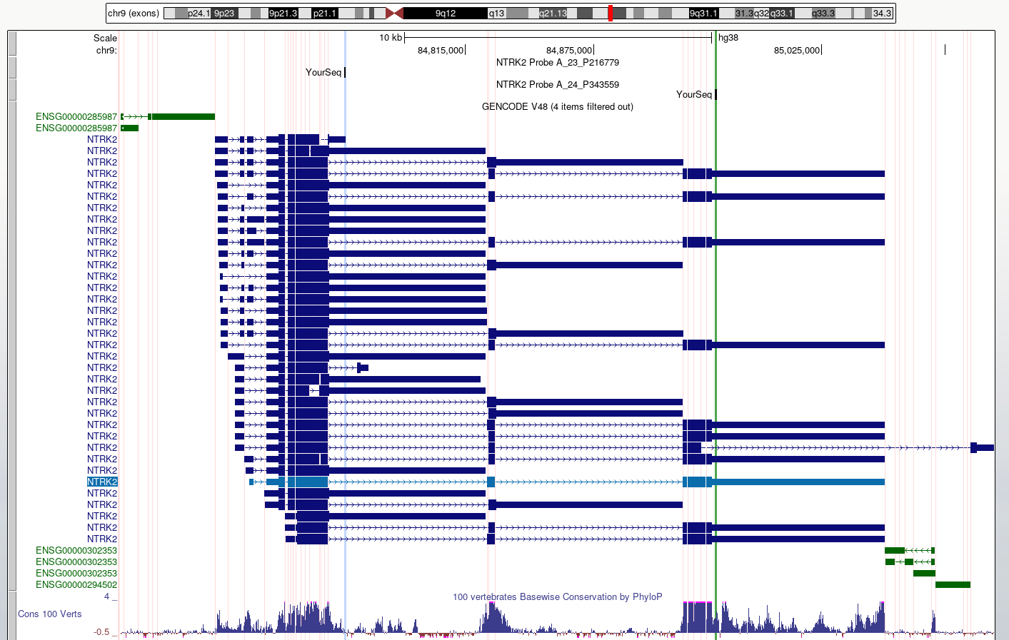
This view makes it easier to check what region
of each transcript is likely to be detected by the probes
UCSC Genome Browser: Gene expression data
Figure 1
Figure 2

Figure 3
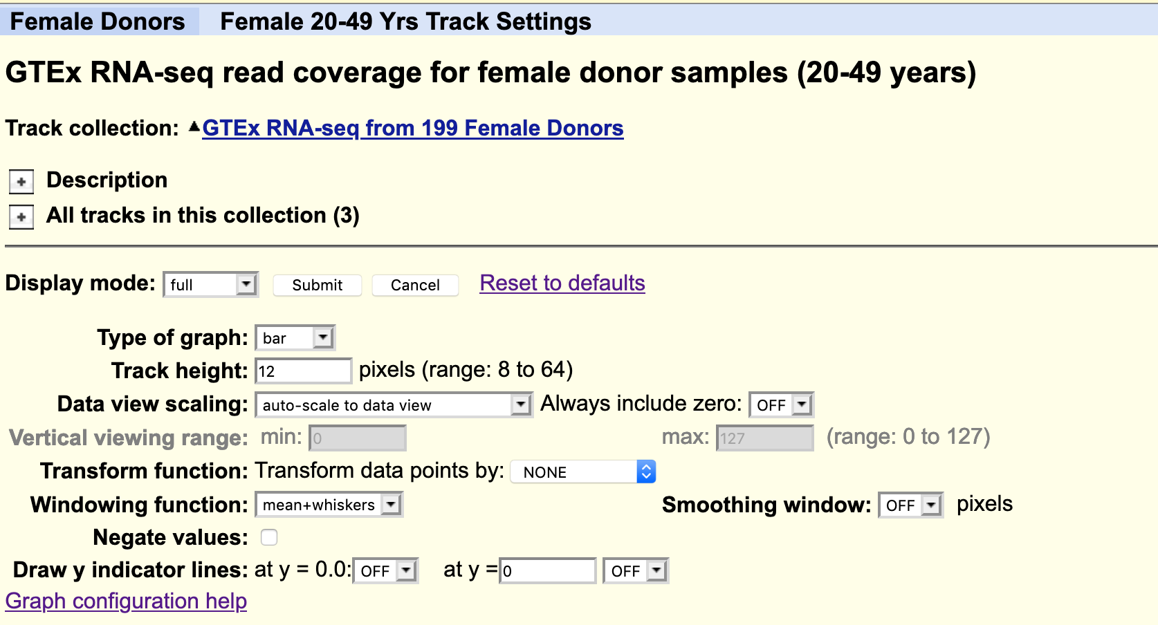
Figure 4
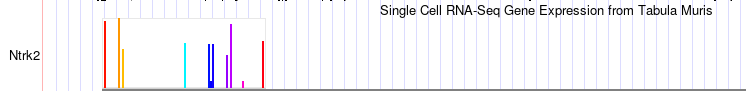
Figure 5
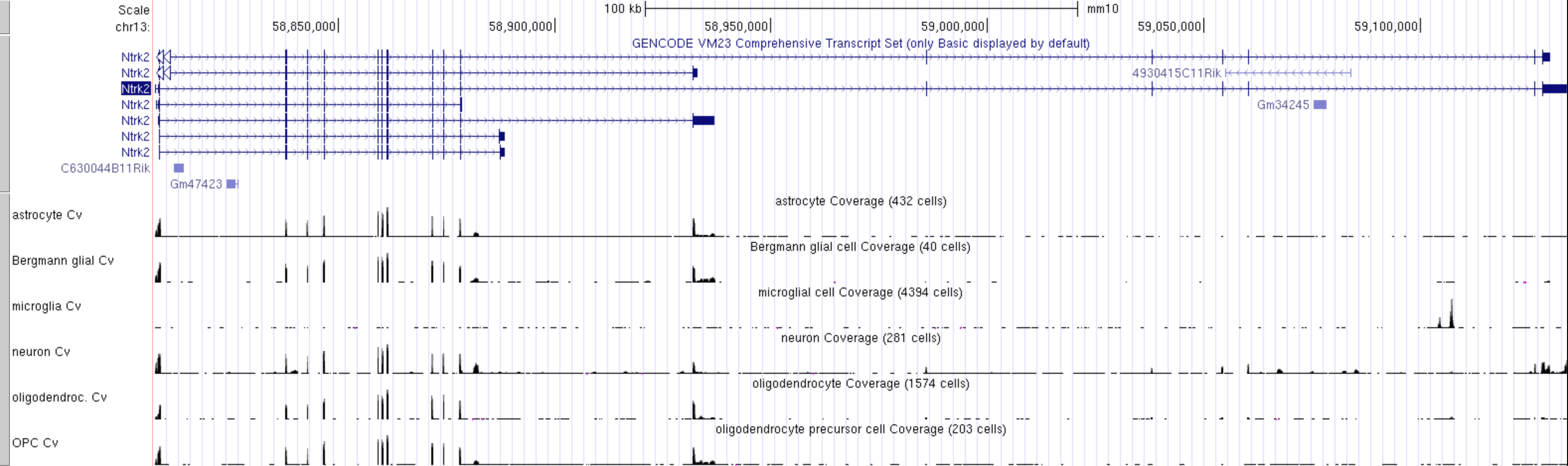
Figure 6
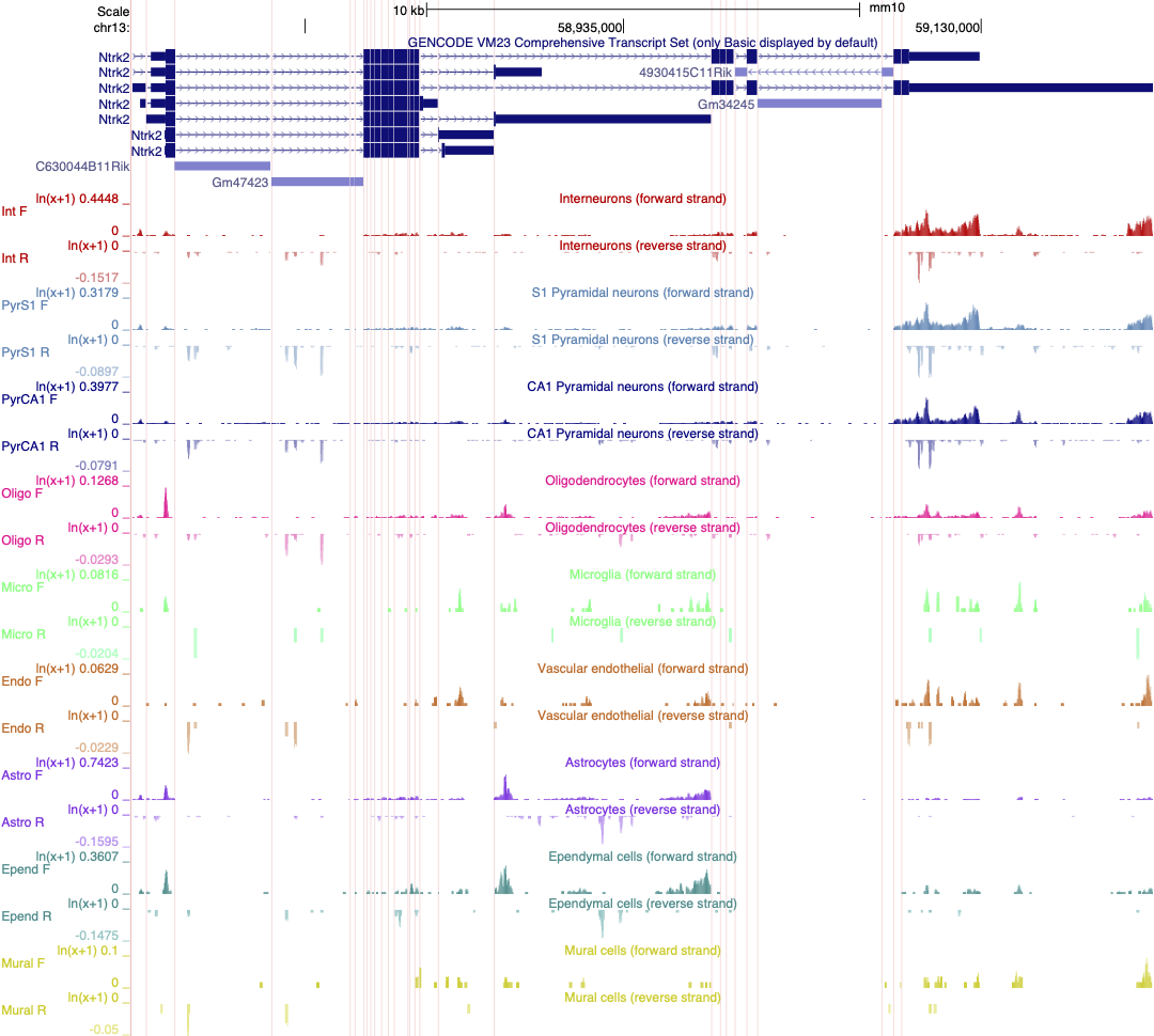
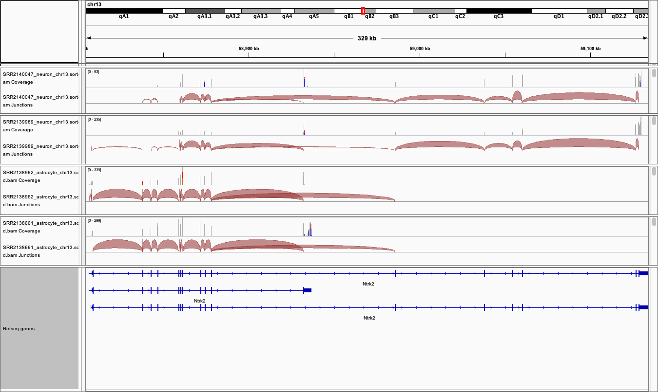
Linnarsson lab mouse cortex single cell data as
autoscaled datatracks
IGV
Figure 1
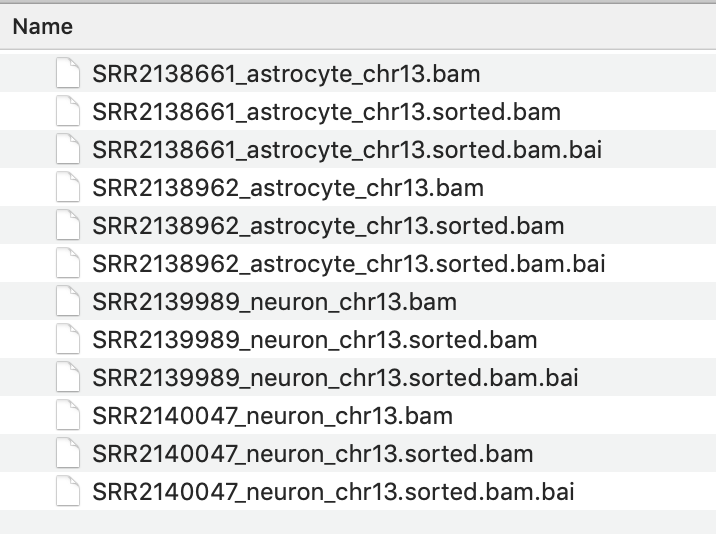
Figure 2
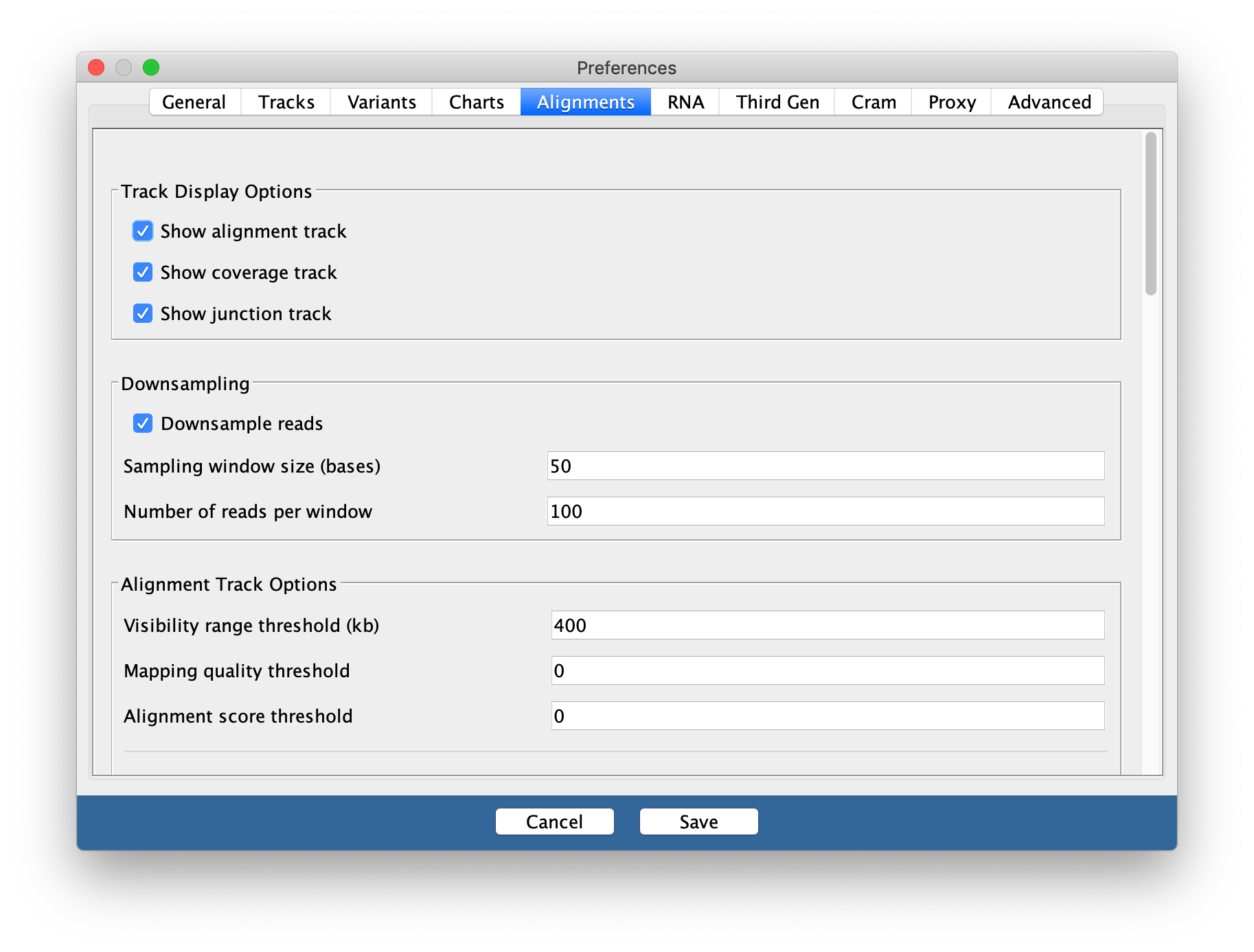
You may need to change this back to a smaller
range in the future if you are working with large datasets and/or small
amounts of memory on your computer
Figure 3